Photonic discrete-time quantum walks [Invited] Download： 901次 | Chinese Optics Letters -- 中国光学期刊网

Chinese Optics Letters, 2020, 18 (5): 052701, Published Online: May. 6, 2020

Photonic discrete-time quantum walks [Invited] Download： 901次

Gaoyan Zhu ^1,2Lei Xiao ^1,2Bingzi Huo ²Peng Xue ^2,*

Author Affiliations

¹ Department of Physics, Southeast University, Nanjing 211189, China

² Beijing Computational Science Research Center, Beijing 100084, China

Figures & Tables

Fig. 1. (a) Experimental setup of one step of a 1D quantum walk. (b) Schematic of N steps of a quantum walk, where module G denotes the setup shown in (a)^[38].

下载图片查看原文

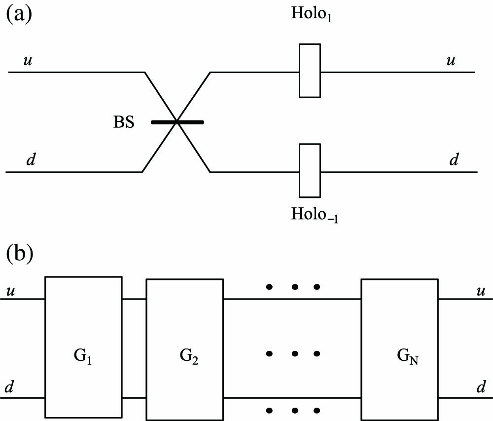
Fig. 2. Schematic of the specially devised OAM beam splitter ( ${BS}^{'}$ ), consisting of a BS (symmetric BS) and two mirrors^[39].

下载图片查看原文

Fig. 3. Experimental scheme of a 1D two-state quantum walk with the specially devised OAM ${BS}^{'}$ . A normal symmetric ${BS}_{1}$ is still used in this scheme, while ${BS}_{2}^{'}$ and ${BS}_{3}^{'}$ are both OAM ${BS}^{'} s$ . Single-mode fibers (SMFs), computer generated holograms with proper $\pm l$ ( ${Holo}_{l}$ ), pinholes ( $P_{1} - P_{6}$ ), and power meters ( $D_{u}$ and $D_{d}$ ) are used for the measurement^[39].

下载图片查看原文

Fig. 4. Conceptual schematic of quantum walks with the spin-orbital system^[41].

下载图片查看原文

Fig. 5. Schematic of the experimental setup to implement 1D quantum walks by using photon SAM as the quantum coin and OAM space as the walk space. A set of three wave-plates [two quarter-wave-plates (QWPs) and one half-wave-plate (HWP)] are used for initial state preparation. The gray box implements one step of quantum walks, consisting of three wave-plates, one QWP and two HWPs, and one $q$ -plate (QP). The OAM analysis module is made up of a computer generated hologram, an SMF, and a single-photon counting module (SPCM)^[42].

下载图片查看原文

Fig. 6. Detailed sketch of the setup for demonstration of a two-particle quantum walk^[41].

下载图片查看原文

Fig. 7. Experimental setup of 2D quantum walks (see text for more details)^[7].

下载图片查看原文

Fig. 8. Schematic of using bulk optics as the basic elements of 1D quantum walks. The $\bar{PBS}$ consists of a PBS and HWPs ( $R_{90}$ ), where a PBS splits the input light into the two output ports denoted by “left” and “right” for $| V 〉$ and $| H 〉$ , respectively^[44].

下载图片查看原文

Fig. 9. Optical layout of the experimental setup for implementing N-step quantum walks on a line^[44].

下载图片查看原文

Fig. 10. Scheme of implementing a quantum quincunx with optical elements^[52].

下载图片查看原文

Fig. 11. Schematic of the experimental demonstration six steps of the quantum walks with single photons. (a) $C_{i}$ and $S_{i}$ indicate six pairs of coin and shift operators, separately. (b) The first two steps are illustrated in detail. (c) Adjusting the relative angle between adjacent BDs, resulting in a temporal lag $Δ t$ and a transversal mode mismatch $Δ x$ between interfering wave-packets, thereby introducing decoherence^[15].

下载图片查看原文

Fig. 12. Experimental results. Probability distributions of the (a) quantum walks and (b) classical walks when introducing decoherence. (c) Normalized standard deviation of the probability distribution, where the lines indicate the theoretical values^[15].

下载图片查看原文

Fig. 13. Experimental setup for realization of quantum walks on cycles with N nodes^[56].

下载图片查看原文

Fig. 14. Detailed schematic of the experimental setup for implementation of arbitrary coined 2D quantum walks (see text for details)^[60].

下载图片查看原文

Fig. 15. (a) Encoding method. The walker’s positions are encoded with the polarization states of single photons. (b) Implementation of the conditional shift operator, where two HWPs at 0° and another two at $Δ θ / 2$ and $- Δ θ / 2$ are used^[63].

下载图片查看原文

Fig. 16. Experimental setup. The photon pairs are generated by the BBO crystal through the SPDC technique, one of which is detected by the single-photon detector ( $D_{0}$ ) as the trigger, while the other one is initialized in the state initialization part and then incident into the optical loops to demonstrate the quantum walks, of which the arrival times can be detected by $D_{1}$ and $D_{2}$ ^[63].

下载图片查看原文

Fig. 17. Schematic setup of the detector. 50:50, symmetric fiber couplers^[64].

下载图片查看原文

Fig. 18. Schematic diagram of the principle of the time-multiplexed framework. The HWP is used to implement the coin flipping operator. The first PBS can separate photons by their polarization to different paths, while the second PBS recombines these photons from different paths to the same one. The red wave indicates the evolution of the first step, and the yellow wave indicates the second step. The arrows represent the direction of polarization.

下载图片查看原文

Fig. 19. Experimental scheme of the time-multiplexed framework^[23].

下载图片查看原文

Fig. 20. (a) Experimental setup. (b) Probability distribution of a Hadamard walk after 28 steps^[24].

下载图片查看原文

Fig. 21. (a) Experimental setup of the 2D quantum walk with one walker. (b) Diagram of a 2D quantum walk separated by two different-direction 1D quantum walks^[25].

下载图片查看原文

Fig. 22. Initial state, produced by a type-II PPKTP crystal, is prepared as a Bell state, and one of the photon pairs is sent to Alice, while the other is sent to Bob. At Alice’s side, projection measurement is implemented to choose the initial state of the system, while Bob that realizes a 2D quantum walk is the same as above. The initial state of Bob can be chosen rather than the beginning of Bob, but not the projection measurement of Alice’s side^[66].

下载图片查看原文

Fig. 23. (a) Experimental setup of 2D time-bin quantum walk. The $x$ direction quantum walk was realized in the fiber loop, while the $y$ direction quantum walk was in the free space loop. The AOM acts as a photo switch to guarantee the effective detection of photons. (b) Reconstruction of 2D quantum walk, where the walker walks along the $x$ direction in step 1, while it walks along the $y$ direction in step 2^[71].

下载图片查看原文

Fig. 24. (a), (b) Probability distribution of 2D quantum walk after 25 steps. (c) $n - P (B; n)$ in different phase parameters. (d) $| d | - 〈 z 〉$ for the parameter of $θ$ in different phases^[71].

下载图片查看原文

Fig. 25. (a) Experimental setup of time-bin quantum walk in the birefringence crystal. (b) Details and the time interval for different steps^[65].

下载图片查看原文

Fig. 26. Normalized probability distribution of Hadamard quantum walk after 50 steps^[65].

下载图片查看原文

Gaoyan Zhu, Lei Xiao, Bingzi Huo, Peng Xue. Photonic discrete-time quantum walks [Invited][J]. Chinese Optics Letters, 2020, 18(5): 052701.

Figures gallery of this article

论文摘要 Full Text 图 & 表补充材料基本信息知识挖掘 Metrics PDF全文参考文献 & 引文

引用该论文： TXT | EndNote

中国光学期刊网使用基于 cookie 的技术来更好地为您提供各项服务，点击此处了解我们的隐私策略。如您需继续使用本网站，请您授权我们使用本地 cookie 来保存部分信息。

您最值得信赖的光电行业旗舰网络服务平台!

快速查询高级查询

最近搜索：

大家在搜：人工智能图像处理光子

热门搜索：机器视觉光通信光纤传感器