High Power Laser Science and Engineering, 2019, 7 (1): 010000e3, Published Online: Jan. 16, 2019
Dynamic stabilization of plasma instability
Figures & Tables
Fig. 1. An example concept of feedback control. (a) At $t=0$ a perturbation is imposed. The initial perturbation may grow at instability onset. (b) After $\unicode[STIX]{x0394}t$ , if the feedback control works on the system, another perturbation, which has an inverse phase with the detected amplitude at $t=0$ , is actively imposed, so that (c) the actual perturbation amplitude is mitigated very well after the superposition of the initial and additional perturbations.
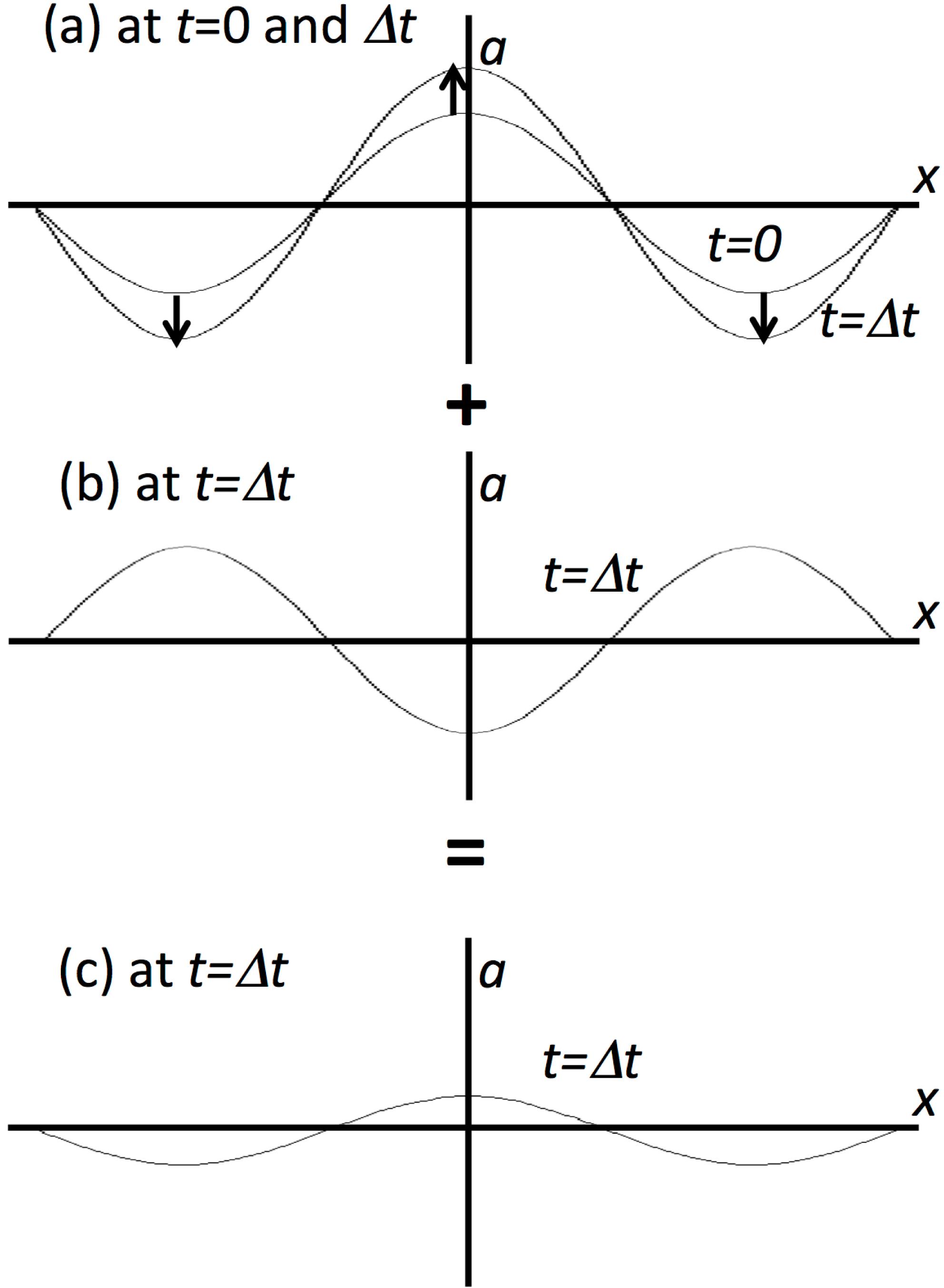
Fig. 2. Kapitza’s pendulum, which can be stabilized by applying an additional strong and rapid acceleration $A\text{sin}\,\unicode[STIX]{x1D714}t$ .

Fig. 3. Superposition of perturbations defined by the wobbling driver beam. At each time the wobbler provides a perturbation, whose amplitude and phase are defined by the wobbler itself. If the system is unstable, each perturbation is a source of instability. At a certain time the overall perturbation is the superposition of the growing perturbations. The superimposed perturbation growth is mitigated by the beam wobbling motion.

Fig. 4. Example simulation results for the Rayleigh–Taylor instability (RTI) mitigation. $\unicode[STIX]{x1D6FF}g$ is 10% of the acceleration $g_{0}$ and oscillates with the frequency of $\unicode[STIX]{x1D6FA}=\unicode[STIX]{x1D6FE}$ . As shown above and in Equation (3 ), the dynamic instability mitigation mechanism works well to mitigate the instability growth.

Fig. 5. Fluid simulation results for the RTI mitigation for the time-dependent $\unicode[STIX]{x1D6FF}g(t)=\unicode[STIX]{x1D6FF}g-\unicode[STIX]{x1D6E5}\sin \unicode[STIX]{x1D6FA}^{\prime }t$ at $t=5/\unicode[STIX]{x1D6FE}$ . In the simulations $\unicode[STIX]{x1D6E5}=0.3$ , and (a) $\unicode[STIX]{x1D6FA}^{\prime }=\unicode[STIX]{x1D6FA}/3$ , (b) $\unicode[STIX]{x1D6FA}^{\prime }=\unicode[STIX]{x1D6FA}$ and (c) $\unicode[STIX]{x1D6FA}^{\prime }=3\unicode[STIX]{x1D6FA}$ . The dynamic mitigation mechanism is robust against the time change of the perturbation amplitude $\unicode[STIX]{x1D6FF}g(t)$ .

Fig. 6. Fluid simulation results for the RTI mitigation for the time-dependent wobbling frequency $\unicode[STIX]{x1D6FA}(t)=\unicode[STIX]{x1D6FA}(1+\unicode[STIX]{x1D6E5}\sin \unicode[STIX]{x1D6FA}^{\prime }t)$ at $t=5/\unicode[STIX]{x1D6FE}$ . In the simulations $\unicode[STIX]{x1D6E5}=0.3$ , and (a) $\unicode[STIX]{x1D6FA}^{\prime }=\unicode[STIX]{x1D6FA}/3$ , (b) $\unicode[STIX]{x1D6FA}^{\prime }=\unicode[STIX]{x1D6FA}$ and (c) $\unicode[STIX]{x1D6FA}^{\prime }=3\unicode[STIX]{x1D6FA}$ . The dynamic mitigation mechanism is also robust against the time change of the perturbation frequency $\unicode[STIX]{x1D6FA}(t)$ .

Fig. 7. Fluid simulation results for the RTI mitigation for the time-dependent wobbling wavelength $k(t)=k_{0}+\unicode[STIX]{x0394}ke^{i\unicode[STIX]{x1D6FA}_{k}^{\prime }t}$ , at $t=5/\unicode[STIX]{x1D6FE}$ . In the simulations $\unicode[STIX]{x0394}k/k_{0}=0.3$ , and (a) $\unicode[STIX]{x1D6FA}_{k}^{\prime }=\unicode[STIX]{x1D6FA}/3$ , (b) $\unicode[STIX]{x1D6FA}_{k}^{\prime }=\unicode[STIX]{x1D6FA}$ and (c) $\unicode[STIX]{x1D6FA}_{k}^{\prime }=3\unicode[STIX]{x1D6FA}$ . The dynamic mitigation mechanism is also robust against the time change of the perturbation wavelength $k(t)$ .

Fig. 8. Filamentation instability. In this case an electron beam has a density perturbation in the transverse direction, and is injected into a plasma. In the plasma return current is induced to compensate for the electron beam current. The perturbed electron beam itself defines the filamentation instability phase, and the e-beam axis oscillates in the $y$ direction in this example case. Therefore, the filamentation instability is mitigated by the dynamic stabilization mechanism.

Fig. 9. Dynamic stabilization mechanism for the filamentation instability. (a) A modulated electron beam is imposed to induce the filamentation instability. The electron beam axis is wobbled or oscillates transversally with its frequency of $\unicode[STIX]{x1D6FA}$ . (b) At a later time its phase-shifted perturbation is additionally imposed by the electron beam itself. The overall perturbation is the superimposition of all the perturbations, and the filamentation instability is dynamically stabilized.

Fig. 10. Filamentation instability simulation results without and with the electron beam oscillation. The current density $J_{x}$ is shown at each time step. When the electron beam axis oscillates in the $y$ direction ((d)–(f) and (g)–(i)), the filamentation instability growth is clearly mitigated.

Fig. 11. Magnetic field $B_{z}$ for the filamentation instability without and with the electron beam oscillation.

Fig. 12. Histories of the normalized magnetic field energy $U_{Bz}\propto |B_{z}|^{2}$ . When the electron beam transverse oscillation frequency $\unicode[STIX]{x1D6FA}$ in $y$ becomes larger than or comparable to $\unicode[STIX]{x1D6FE}_{F}$ , the dynamic stabilization effect is remarkable.

Fig. 13. 3D PIC simulation results for the filamentation instability growth at (a) $t=0$ and (b) $t=32\unicode[STIX]{x1D714}_{pe}$ without the electron beam wobbling motion, and (c) $t=0$ and (d) $t=32\unicode[STIX]{x1D714}_{pe}$ with the wobbling motion. The histories of the normalized magnetic field energy $U_{Bz}\propto |B_{z}|^{2}$ is shown in (e). When the electron beam transverse oscillation frequency $\unicode[STIX]{x1D6FA}$ in $y$ becomes larger than or comparable to $\unicode[STIX]{x1D6FE}_{F}$ , the dynamic stabilization effect is also remarkable. The 3D simulation results also confirm the instability mitigation mechanism in the plasma.

S. Kawata, T. Karino, Y. J. Gu. Dynamic stabilization of plasma instability[J]. High Power Laser Science and Engineering, 2019, 7(1): 010000e3.


 PDF全文
PDF全文

