Spatial cage solitons—taming light bullets

Chao Mei; Ihar Babushkin; Tamas Nagy; Günter Steinmeyer

doi:doi:10.1364/PRJ.438610

Photonics Research, 2022, 10 (1): 01000148, Published Online: Dec. 14, 2021

Spatial cage solitons—taming light bullets Download： 556次

Chao Mei ^1,2Ihar Babushkin ³Tamas Nagy ¹Günter Steinmeyer ^1,4,*

Author Affiliations

¹ Max Born Institute for Nonlinear Optics and Short Pulse Spectroscopy, 12489 Berlin, Germany

² School of Computer and Communication Engineering, University of Science and Technology Beijing (USTB), Beijing 100083, China

³ Institute of Quantum Optics, Leibniz University Hannover, 30167 Hannover, Germany

⁴ Institut für Physik, Humboldt Universität zu Berlin, 12489 Berlin, Germany

Figures & Tables

Fig. 1. (a) Mode fields of the first four EH1n modes considered in this study. Intensities are depicted by colors, and electric fields are represented by arrows. (b) Ray-optical representation of hollow-fiber transmission. The wave vector k0 can be decomposed into a transverse component k⊥ and a longitudinal component β, which are connected by Pythagoras’ theorem [38]. (c) The propagation constants βn of the individual EH1n modes follow an approximate n2 dependence, whereas the k⊥,n underly a linear relationship with n. (d) Intramode dispersion, deviation of the propagation constants of the first 10 EH1n modes from the propagation constant of a plane wave, calculated at 800 nm wavelength for an HCF with a core radius of 100 μm; symbols, exact solution according to Eq. (3); curve, parabolic fit; the four modes of interest within this study are highlighted in red, indicating a dephasing of ≈8 rad/cm in the linear optical regime.

下载图片查看原文

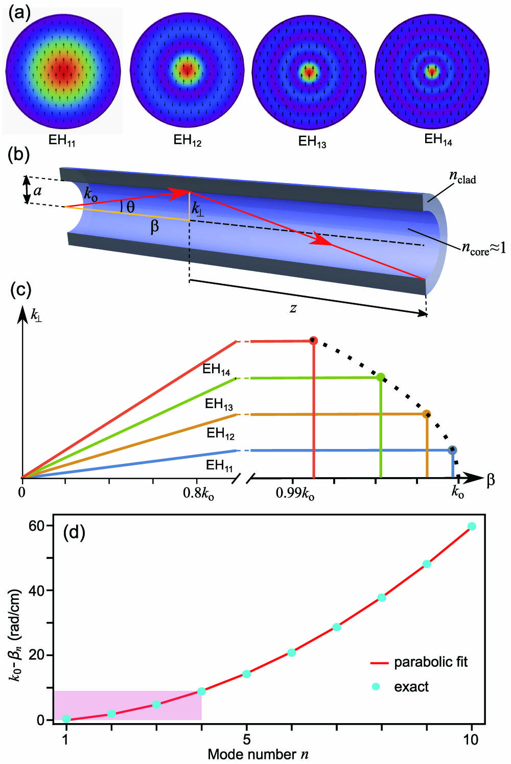
Fig. 2. Spatial soliton solution branches of Eq. (8). For normal modal dispersion (ncore>nclad), a single solution branch exists (green). In hollow fibers, two branches coexist (blue and red). The red branch is considered unstable (see discussion in text). (a) Radially integrated intensity ∫E(r)2rdr=P of the spatial cage soliton solutions versus effective nonlinearity. Powers have been normalized to the critical power of self-focusing Pcr in free space [9]. Insets show E(r) for parameters indicated by symbols. (b) Root mean square mode diameter of spatial solitons normalized to the HE11 mode; insets show spatial intensity profiles |E(r)|2.

下载图片查看原文

Fig. 3. Three-dimensional visualization of the light bullet structure at the stability limit (≈1.4Pcr) in the anomalous modal dispersion regime. Equi-intensity surfaces are shown with colors red (80% peak intensity) to blue (10% peak intensity). In the center, a donut structure dominates, which evolves into an ellipsoidal shape in the temporal wings. The glass–gas interface of the hollow fiber is depicted in light gray for comparison.

下载图片查看原文

Fig. 4. Comparison of model results with measured data. (a) Total losses (linear and nonlinear) versus ratio of a3 and λ2 (curve and red dots). Early measurements with relatively short hollow fibers exhibited significantly higher losses, whereas more recent measurements showed excellent agreement as indicated by the respective references [19 21" target="_self" style="display: inline;">–21]. (b) Maximum beneficial length (solid curve and hollow triangles) and maximum compressibility (dashed line and solid triangles); cf. Eq. (13). This analysis confirms that superior compression can be reached with longer hollow fibers and larger core diameters.

–21]. (b) Maximum beneficial length (solid curve and hollow triangles) and maximum compressibility (dashed line and solid triangles); cf. Eq. (13). This analysis confirms that superior compression can be reached with longer hollow fibers and larger core diameters." class="imgSplash img-thumbnail" style="cursor:pointer;">

下载图片查看原文

Table1. Nonlinear Mode-Coupling Factors^a

XPM	$η_{12} = 1.709$	$η_{13} = 1.529$	$η_{14} = 1.408$
XPM	$η_{23} = 1.847$	$η_{24} = 1.725$	$η_{34} = 1.897$
FWM	$η_{123} = 0.788$	$η_{234} = 0.874$	$η_{1234} = 1.462$

查看原文

Chao Mei, Ihar Babushkin, Tamas Nagy, Günter Steinmeyer. Spatial cage solitons—taming light bullets[J]. Photonics Research, 2022, 10(1): 01000148.

Spatial cage solitons—taming light bullets Download： 556次

Table1. Nonlinear Mode-Coupling Factors^a

关于本站 Cookie 的使用提示

全站搜索

Spatial cage solitons—taming light bullets Download： 556次

Table1. Nonlinear Mode-Coupling Factorsa

相关论文

相关资讯

关于本站 Cookie 的使用提示

全站搜索

Table1. Nonlinear Mode-Coupling Factors^a