光场相干测量及其在计算成像中的应用

张润南; 蔡泽伟; 孙佳嵩; 卢林芃; 管海涛; 胡岩; 王博文; 周宁; 陈钱; 左超

doi:doi:10.3788/LOP202158.1811003

激光与光电子学进展, 2021, 58 (18): 1811003, 网络出版: 2021-09-02

光场相干测量及其在计算成像中的应用下载： 5986次内封面文章特邀综述

Optical-Field Coherence Measurement and Its Applications in Computational Imaging

张润南 ^1,2,3蔡泽伟 ^1,2,3,**孙佳嵩 ^1,2,3卢林芃 ^1,2,3管海涛 ^1,2,3胡岩 ^1,2,3王博文 ^1,2,3周宁 ^1,2,3陈钱 ^3,***左超 ^1,2,3,*

作者单位

¹ 智能计算成像实验室, 南京理工大学电子工程与光电技术学院, 江苏南京210094

² 南京理工大学智能计算成像研究院, 江苏南京210019

³ 江苏省光谱成像与智能感知重点实验室, 江苏南京 210094

图 & 表

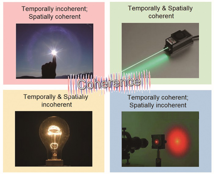
图 1. 光源的时间相干性与空间相干性的若干典型实例

Fig. 1. Several typical examples of light sources with different degrees of temporal coherence and spatial coherence

下载图片查看原文

图 2. 光信号在时间与空间上的表示形式。(a)光信号是空间上确定一点的关于时间的函数;(b)光信号是时间上确定一点的关于空间的函数

Fig. 2. Representation of optical signal in time and space. (a) Optical signal is a function of time at a certain point in space; (b) optical signal is a function of space at a certain point in time

下载图片查看原文

图 3. 不同频率光波的叠加。(a)不同频率的光波相干叠加为一个脉冲波包;(b)不同频率的光波非相干叠加为一个连续波(非周期无限宽),其相位与振幅都是随机变化的

Fig. 3. Superposition of light waves with different frequencies. (a) Waves with different frequencies are coherently superimposed into one pulse wave packet; (b) waves with different frequencies are incoherently superimposed into one continuous wave (non-periodic and infinite width), and its phase and amplitude vary randomly

下载图片查看原文

图 4. 傅里叶变换光谱仪的基本原理

Fig. 4. Basic principle of Fourier transform spectrometer

下载图片查看原文

图 5. 迈克耳孙恒星干涉仪通过干涉法来测量准单色光场的空间相干度,反推出光源的尺寸。(a) 光路示意图;(b) 系统实物图

Fig. 5. Michelson stellar interferometer measures the spatial coherence of a quasi-monochromatic wave field by interferometry to infer the size of the light source. (a) Optical configuration; (b) photograph of a real system

下载图片查看原文

图 6. 经典相干理论与相空间光学的关联

Fig. 6. Relationship between classical coherence theory and phase space optics

下载图片查看原文

图 7. 常见信号变换在相空间的表征。(a)菲涅耳传播;(b) Chirp调制(透镜);(c)傅里叶变换;(d)分数阶傅里叶变换;(e) 光束放大器

Fig. 7. Characterization of common signal transformations in phase space. (a) Fresnel propagation; (b) Chirp modulation (lens); (c) Fourier transform; (d) fractional Fourier transform; (e) magnifier

下载图片查看原文

图 8. 特殊信号的Wigner分布示意图。(a)点光源;(b)平面波;(c)球面波;(d)相位缓变波;(e)高斯信号

Fig. 8. Wigner distribution function of special signals. (a) Point source; (b) plane wave; (c) spherical wave; (d) phase slow-varying wave; (e) Gaussian signal

下载图片查看原文

图 9. 光场的参数化表征。(a)七维全光函数;(b)双平行平面四维光场;(c)位置角度式四维光场

Fig. 9. Parameterization of the light field. (a) Seven-dimensional plenoptic function; (b) two planes parameterization of four-dimensional light field; (c) position-angular parameterization of four-dimensional light field

下载图片查看原文

图 10. 光滑相干波前的Wigner分布函数和光场的关系^[128]。相位对应Wigner分布函数中的局部空间频率(瞬时频率),光线垂直于波前方向传播(相位的法线方向)。(a)空域中的波前;(b)相空间中的Wigner分布函数;(c)在位置-角度空间的光场

Fig. 10. Relationship between Wigner distribution function and light field of a smooth coherent wavefront. Phase is represented as the localized spatial frequency (instantaneous frequency) in the Wigner distribution function. Rays travel perpendicularly to the wavefront (phase normal)^[128]. (a) Wavefront in real space; (b) Wigner distribution function in phase space; (c) light field in position-angle space

下载图片查看原文

图 11. 相位成像技术的分类

Fig. 11. Classification of phase imaging techniques

下载图片查看原文

图 12. 相干测量技术分类

Fig. 12. Classification of the coherence measurement techniques

下载图片查看原文

图 13. 杨氏双孔干涉法^[22]

Fig. 13. Young’s interferometry with two holes^[22]

下载图片查看原文

图 14. 逆波前杨氏干涉法^[77]

Fig. 14. Reversed-wavefront Young’ interferometry^[77]

下载图片查看原文

图 15. 非冗余孔径阵列布局和实验装置示意图^[78]。 (a1)轴上点占优;(a2)点中心分布;(a3)轴外点占优;(b)非冗余孔径实验示意图

Fig. 15. Distributions of nonredundant array method and experimental scheme^[78]. (a1) Superior in points on axes; (a2) central distribution of points; (a3) superior in points out of axes; (b) experimental scheme of nonredundant array method

下载图片查看原文

图 16. 自参考干涉法实验示意图^[80]

Fig. 16. Experimental scheme of self-referencing interferometry^[80]

下载图片查看原文

图 17. Wigner分布函数和模糊函数的对应关系

Fig. 17. Correspondence between Wigner distribution function and ambiguity function

下载图片查看原文

图 18. 相空间断层扫描原理示意图。(a)垂直投影;(b)旋转四分之一投影;(c)旋转90°投影;(d)各角度投影叠加

Fig. 18. Basic principle of phase space tomography. (a) Vertical projection; (b) quarter rotation projection; (c) rotation by 90° projection; (d) superposition of all projections from different angles

下载图片查看原文

图 19. 实现相空间断层扫描的两种Wigner分布函数(WDF)变换。(a) 复信号的WDF;(b) 菲涅耳衍射后的WDF表示;(c) 分数阶傅里叶变换后的相空间WDF表示;(d) 菲涅耳衍射与分数阶傅里叶变换的对应关系

Fig. 19. Two different transformations of WDF for phase space tomography. (a) WDF of complex signal; (b) WDF after Fresnel diffraction; (c) phase space WDF after fractional Fourier transform; (d) correspondence between Fresnel diffraction and fractional Fourier transform

下载图片查看原文

图 20. 相空间断层扫描的光路结构^[85]

Fig. 20. Optical path structure of phase space tomography^[85]

下载图片查看原文

图 21. 基于边缘衍射测量空间相干性的实验装置^[84]

Fig. 21. Experimental device for measuring spatial coherence based on edge diffraction^[84]

下载图片查看原文

图 22. 相空间的直接测量。(a) 基于小孔扫描的相空间直接测量; (b)基于微透镜阵列的相空间直接测量

Fig. 22. Direct phase space measurement. (a) Direct phase space measurement based on pinhole scanning; (b) direct phase space measurement based on microlens array

下载图片查看原文

图 23. 相干光场和部分(空间)相干光场的简化示意图。 (a)相干光场由二维复振幅表示,几何光线垂直于波前传播,恒定相位面即为波前;(b)部分相干光场需要四维相干函数以准确地表示其传播和衍射等特性。部分相干光场的“相位”(广义相位)是空间中每个位置的相位(空间频率,传播方向)的统计集合

Fig. 23. Schematic of a simplistic view of coherent field and partially (spatially) coherent field. (a) A coherent field requires a 2D complex amplitude representation, the surface of the constant phase is interpreted as wavefronts with geometric light rays traveling normal to them; (b) a partially coherent field requires a 4D coherence function to accurately represent its properties such as propagation and diffraction. The “phase” (generalized phase) of a partially coherent light field is the statistical average of phases (spatial frequency, direction of propagation) at each position in space

下载图片查看原文

图 24. 夏克-哈特曼波前传感器和光场相机的原理。(a) 对于相干场,夏克-哈特曼波前传感器的信号为焦点阵列;(b) 对于部分相干场,夏克-哈特曼波前传感器的信号扩展为光源阵列;(c) 对于非相干成像,光场照相机产生的信号为二维子孔径图像阵列

Fig. 24. Principle of the Shack-Hartmann sensor and light field camera. (a) For coherent field, the Shack-Hartmann sensor forms a focus spot array sensor signal; (b) for partially coherent field, the Shack-Hartmann sensor forms an extended source array sensor signal; (c) for incoherent imaging, the light field camera produces a 2D sub-aperture image array

下载图片查看原文

图 25. 光场成像技术分类

Fig. 25. Classification of light field imaging techniques

下载图片查看原文

图 26. 基于相机阵列的光场采集。(a)搭建的光场龙门架^[126]; (b)大规模相机阵列^[110];(c)5×5相机阵列实现显微光场采集^[189]

Fig. 26. Light field capture based on camera arrays. (a) Light field gantry^[126]; (b) large camera arrays^[110]; (c) micro light field acquisition acquired by the 5×5 camera array system^[189]

下载图片查看原文

图 27. 各种基于微透镜阵列的光场相机系统

Fig. 27. Various light field cameras based on microlens array

下载图片查看原文

图 28. 基于编码掩模的计算光场成像。 (a)掩模增强相机光场采集^[191];(b)压缩光场采集^[192]

Fig. 28. Computational light field imaging based on coded mask. (a) Light field acquisition of mask enhanced camera^[191]; (b) light field acquisition of compressive photography^[192]

下载图片查看原文

图 29. 基于可编程孔径的光场成像。 (a)可编程孔径光场相机^[104];(b)可编程孔径光场显微镜^[106]

Fig. 29. Light field imaging based on programmable aperture. (a) Programmable aperture light field camera^[104]; (b) programmable aperture light field microscope^[106]

下载图片查看原文

图 30. 缓变物体在空域平稳照明下的光场表示^[128]

Fig. 30. Light field representation of a slowly varying object under spatially stationary illumination^[128]

下载图片查看原文

图 31. 光场显微镜模型。(a)传统明场显微镜;(b)光场显微镜^[111];(c)基于波动光学的光场显微模型^[112];(d)傅里叶光场显微镜模型^[113]

Fig. 31. Light field microscope model. (a) Traditional bright field microscope; (b) light field microscope^[111]; (c) light field microscopic model based on wave optics theory^[112]; (d) Fourier light field microscope^[113]

下载图片查看原文

图 32. 光强传输方程与弱物体传递函数对比^[207]。(a1)(b1) 光强传输方程和弱物体传递函数的物理含义;(a2)(b2)推导相位梯度传递函数和弱物体传递函数的几何图解;(a3)(b3) 相位梯度传递函数和弱物体传递函数在不同s下的相位成像

Fig. 32. Comparison between TIE and WOTF^[207]. (a1)(b1) Physical implications of TIE and WOTF; (a2)(b2) geometric illustrations for deriving the PGTF and WOTF; (a3)(b3) PGTF and WOTF for phase imaging under different s

下载图片查看原文

图 33. 由相干全息图重建的相干图像的直接可视化^[209]

Fig. 33. Direct visualization of coherent images reconstructed from coherent holograms^[209]

下载图片查看原文

图 34. 光子相关全息术^[213]。(a) 光子相关全息术的概念图;(b)光强干涉仪原理图

Fig. 34. Photon correlation holography^[213]. (a) Concept diagram of photon-dependent holography; (b) schematic diagram of intensity interferometer

下载图片查看原文

图 35. 典型的非相干全息光路图。 (a)改进的三角全息干涉光路^[217];(b)菲涅耳非相干关联全息术光路^[214];(c)迈克耳孙干涉仪^[119];(d)Sagnac干涉仪^[215];(e)Mach-Zehnder干涉仪^[216,218]

Fig. 35. Representative optical setup for incoherent holography. (a) Optical path of modified triangular interferometer^[217]; (b) optical path of FINCH^[214]; (c) Michelson interferometer^[119]; (d) Sagnac interferometer^[215]; (e) Mach-Zehnder interferometer^[216,218]

下载图片查看原文

图 36. 编码孔径相关全息的典型光路结构。(a)编码孔径相关全息结构^[115];(b)无干涉编码孔径相关全息结构^[117];(c)无透镜非干涉编码孔径相关全息结构^[116]

Fig. 36. Typical imaging optical path for COACH. (a) Structure of COACH^[115]; (b) structure of I-COACH^[117]; (c) structure of LI-COACH^[116]

下载图片查看原文

图 37. 透过强散射层非入侵式散射成像示意图^[237]

Fig. 37. Schematic of non-invasive scattering imaging through strong scattering layers^[237]

下载图片查看原文

图 38. 基于单帧散斑自相关的透过强散射层成像^[238]。 (a)实验装置模型;(b)相机原始图像;(c)自相关;(d)通过迭代相位恢复算法重建物体;(e)实验系统;(f)相机原始数据;(g)~(k)第一列为自相关,第二列为重建物体,第三列为真实的物体

Fig. 38. Single frame imaging based on speckle autocorrelation through strong scattering layer^[238]. (a) Experimental setup; (b) raw camera image; (c) autocorrelation; (d) image reconstructed by an iterative phase-retrieval algorithm; (e) photograph of the experiment; (f) raw camera image; (g)--(k) Left column is calculated autocorrelation, middle column is reconstructed object; right column is image of the real object

下载图片查看原文

图 39. 传统非相干合成孔径系统结构。(a)迈克耳孙型干涉仪;(b)中次镜结构;(c)相控阵列结构

Fig. 39. Conventional incoherent synthetic aperture structure. (a) Michelson interferometer; (b) common secondary structure; (c) multiple telescopes structure

下载图片查看原文

图 40. 初代SPIDER成像概念系统设计模型。(a)SPIDER设计模型和爆炸图;(b)两个物理基线和三个光谱波段的PIC示意图;(c)SPIDER微透镜排列方式;(d)对应排列方式下频谱覆盖

Fig. 40. Design model of the initial generation of SPIDER imaging conceptual system. (a) Explosive view of SPIDER; (b) PIC schematics of the two physical baselines and three spectral bands; (c) arrangement of SPIDER microlens; (d) corresponding frequency-spectrum coverage

下载图片查看原文

图 41. 基于FINCH的非相干合成孔径技术^[243]

Fig. 41. Incoherent synthetic aperture technology based on FINCH^[243]

下载图片查看原文

图 42. 可见锥束层析的旋转剪切干涉仪实验装置^[79]

Fig. 42. RSI of visible cone-beam tomography^[79]

下载图片查看原文

图 43. 光场显微在生物科学中的应用。(a)小鼠头戴MiniLFM^[252];(b)使用HR-LFM成像COS-7活细胞中的高尔基源膜泡^[74]; (c)DAOSLIMIT观测小鼠肝脏中中性粒细胞迁移过程^[73];(d)共聚焦光场显微镜观测斑马鱼的捕猎活动和小鼠大脑的神经活动^[75]

Fig. 43. Application of light field microscopy in bioscience.(a) Mouse with a head-mounted MiniLFM^[252]; (b) imaging Golgi-derived membrane vesicles in living COS-7 cells using HR-LFM ^[74]; (c) dynamics during neutrophil migration in mouse liver using DAOSLIMIT^[73]; (d) hunting activity of zebrafish and the neural activity of mouse brain observed by confocal light field microscope^[75]

下载图片查看原文

图 44. 基于菲涅耳非相干关联全息术的显微成像。(a)FINCHSCOPE原理图;(b) FINCHSCOPE对花粉成像^[118];(c) TLCGRIN对花粉粒的重建结果,并与相同显微镜的宽视野图像进行对比,利用20× (0.75 NA)物镜^[253];(d)用宽视场(左)和FINCH(右)比较HeLa细胞中三种不同高尔基体蛋白的成像^[255]

Fig. 44. Microscopy imaging based on FINCH. (a) FINCHSCOPE schematic; (b) FINCHSCOPE fluorescence sections of pollen grains^[118]; (c) wide-field image and reconstructed FINCH image of pollen grains captured using a 20×(0.75 NA) objective^[253]; (d) comparative imaging of three different Golgi apparatus proteins in HeLa cells using wide-field (left) and FINCH(right)^[255]

下载图片查看原文

图 45. 光场成像在计算摄像的应用。(a) 光场重聚焦^[101]; (b) 基于光场的合成孔径成像^[259]

Fig. 45. Light field imaging in computational photography. (a) Light field refocusing^[101]; (b) synthetic aperture imaging based on light field^[259]

下载图片查看原文

图 46. 基于菲涅耳非相干关联全息术的计算摄影重聚焦。(a)菲涅耳非相干关联全息术对物体数字的重聚焦结果^[214];(b)彩色全息图数字重聚焦^[260];(c)自然光照明下全彩全息数字重聚焦^[119]

Fig. 46. Computational photography refocusing based on FINCH. (a) Digital refocusing based on FINCH^[214]; (b) colorful digital holography refocusing^[260]; (c) full color holographic digital refocusing under natural light illumination^[119]

下载图片查看原文

图 47. 相空间层析成像的X射线表征。(a) 测量X射线的强度分布,作为横向位置和沿传播方向的函数;(b)由图47(a)中的数据重构的相空间密度^[263];(c)(d)在两种情况下测量的光束的复相干度^[263]

Fig. 47. X-ray characterization via phase space tomography. (a) Measured intensity distribution of the X rays as a function of lateral position and along the direction of propagation^[263]; (b) phase space density reconstructed from the data in Fig.47(a); (c)(d) measured complex degree of coherence for the beams in the two conditions^[263]

下载图片查看原文

图 48. 相空间断层扫描表征光束。(a)一维信号^[265];(b)笛卡儿坐标系可分离光束^[264];(c)旋转对称光束^[266];(d) 不同相干度光束的强度分布(第一行),光束Wigner分布函数呈现出与其相干态相关的隐藏差异(第二行)^[267]

Fig. 48. Optical beam characterization via phase space tomography. (a) 1D signal^[265]; (b) optical beams separable in Cartesian coordinates^[264]; (c) rotationally symmetric beams^[266]; (d) intensity distributions of the test beams with different degrees of coherence (first row), the Wigner distribution function of the beams exhibits hidden differences associated with their coherence state (second row)^[267]

下载图片查看原文

图 49. 相位恢复和因子M²计算示意图^[268]。(a)(b)两个不同纵向位置的轴向强度图像;(c)TIE相位恢复;(d)任何选定平面上的重建强度分布;(e)对光束宽度进行双曲线拟合,并计算M²

Fig. 49. Schematic diagram of phase retrieval and factor M² calculation^[268]. (a)(b) Axial intensity images at two different longitudinal positions; (c) phase retrieval by TIE; (d) reconstructed intensity distribution at any selected plane; (e) performing a hyperbolic fit to the beam widths and calculating the M²

下载图片查看原文

图 50. 在不同数值孔径下,通过光场重心直接恢复相位^[128]。(a) 0.05;(b) 0.15;(c) 0.2;(d) 0.25

Fig. 50. Under different numerical apertures, the phase is recovered directly through the gravity of the light field^[128]. (a) 0.05; (b) 0.15; (c) 0.2; (d) 0.25

下载图片查看原文

图 51. 部分相干照明下,有无模式分解法恢复的相位^[269]

Fig. 51. Reconstructed phases with and without mode decomposition method under partially coherent illumination^[269]

下载图片查看原文

图 52. 基于相干模式分解的叠层成像。(a)散射成像中的相干退化^[270];(b)单模式和多模式复用的傅里叶叠层成像实验方案^[271]

Fig. 52. Stack imaging based on coherent mode decomposition. (a) Decoherence in scattering imaging^[270];(b) experimental scheme of Fourier stack imaging with single-mode and multi-mode multiplexing^[271]

下载图片查看原文

图 53. 基于菲涅耳非相干关联全息术的合成孔径技术。(a)~(c) SLM加载的三种相位函数;(d)单孔径重建结果;(e)多孔径合成重建结果^[243];(f)传统成像系统获得的图像;(g)360×360菲涅耳非相干关联全息术系统产生的全息图对应的重建像;(h)双透镜菲涅耳非相干关联全息术合成孔径产生的全息图对应的重建像;(i)1080×1080菲涅耳非相干关联全息术系统产生的全息图对应的重建像^[275]

Fig. 53. Synthetic aperture technique based on FINCH. (a)--(c) Three phase functions loaded on SLM; (d) single aperture reconstruction result; (e) synthetic multi aperture reconstruction result^[243]; (f) image obtained by the conventional imaging system; (g) reconstructed image corresponding to the hologram produced by the 360×360 FINCH system; (h) reconstructed image corresponding to the hologram produced by synthetic aperture of double lens FINCH; (i) reconstructed image corresponding to the hologram produced by the 1080×1080 FINCH system^[275]

下载图片查看原文

图 54. SPIDER成像实验结果^[277]。(a)搭建的PIC图像实验台;(b)迭代算法得到的关于图54(g)的重建结果;(c)(g)用于实验的两个目标图像;(d)(h)对应目标图像的原理仿真结果;(e)(i)傅里叶逆变换重建得到的成像结果;(f)(j)矫正转台摆动误差后,傅里叶逆变换重建得到的成像结果

Fig. 54. Experimental results of SPIDER imaging^[277]. (a) PIC image experimental platform; (b) iterative image reconstruction result of Fig.54(g); (c)(g) two images of the target; (d)(h) corresponding principle simulation results of target image; (e)(i) imaging results obtained by inverse Fourier transform reconstruction; (f)(j) after correcting the swing error of the turntable, the imaging results are reconstructed by inverse Fourier transform

下载图片查看原文

图 55. 无透镜非干涉编码孔径相关全息^[116]。(a)两颗LEDs;(b)两个硬币

Fig. 55. Lensless noninterference coded aperture dependent holography^[116]. (a) Two LEDs; (b) two one-dime coins

下载图片查看原文

图 56. 基于菲涅耳区域光阑的非相干无透镜成像。 (a) 无镜头相机的实时图像捕获和重建^[279];(b) 利用菲涅耳区域光阑单帧无透镜相机对二值、灰度和彩色图像进行重建^[282]

Fig. 56. Incoherent lensless imaging based on Fresnel region aperture. (a) Real time image capture and reconstruction of lens less camera^[279]; (b) binary, gray, and color images are reconstructed by Fresnel region aperture single frame lensless camera^[282]

下载图片查看原文

表 1光学相干性量度:经典相干理论与相空间光学理论

Table1. Coherence measurement: classical coherence theory and phase space optics theory

Theory	Function	Definition	Temporal/Spatial coherence
Classical coherence theory	Mutual coherence function	Γ(x₁,x₂,τ)=<U(x₁,t)U^*(x₂,t+τ)>	Temporal and spatial
	Complex degree of coherence	γ(x₁,x₂,τ)= $\frac{Γ (x_{1}, x_{2}, τ)}{{[Γ (x_{1}, x_{1}, 0) Γ (x_{2}, x_{2}, 0)]}^{1 / 2}}$
	Cross-spectral density function	W(x₁,x₂,ω)=∫Γ(x₁,x₂,τ)exp(2πiντ)dτ
	Self-coherence function	Γ(x,τ)=<U(x,t)U^*(x,t+τ)>Note: I(x)=Γ(x,0)	Temporal
	Self complex degree of coherence function	γ(x,τ)= $\frac{Γ (x, τ)}{Γ (x, 0)}$	Temporal
	Mutual intensity	J(x₁,x₂)≡Γ(x₁,x₂,0)=<U(x₁,t)U^*(x₂,t)>	Spatial quasi-monochromatic
	Complex coherence factor	j(x₁,x₂)≡γ(x₁,x₂,0)= $\frac{J (x_{1}, x_{2})}{{[J (x_{1}, x_{1}) J (x_{2}, x_{2})]}^{1 / 2}}$	Spatial quasi-monochromatic
Phase space optics theory	Wigner distribution function	W(x,u)=∫W $(x + \frac{x'}{2}, x - \frac{x'}{2})$ exp(-j2πux')dx'=∫Γ $(u + \frac{u'}{2}, u - \frac{u'}{2})$ exp(j2πxu')du'	Spatial
Phase space optics theory	Ambiguity function	A(u',x')=∫W $(x + \frac{x'}{2}, x - \frac{x'}{2})$ exp(-j2πux')dx=∫Γ $(u + \frac{u'}{2}, u - \frac{u'}{2})$ exp(j2πux')du	Spatial

查看原文

表 2Wigner分布函数的性质

Table2. Properties of Wigner distribution function

Property	Representation	Explanation
Realness	W(x,u)∈ℝ	W is always a real function
Spatial marginal property	I(x)=∫W(x,u)du	I(x) is the intensity
Spatial frequency marginal property	S(u)=∫W(x,u)dx	S(u) is the power spectrum
Convolution property	U(x)=U₁(x)U₂(x) W(x,u)=W₁(x,u) $\underset{u}{\otimes}$ W₂(x,u)U(x)=U₁(x) $\underset{x}{\otimes}$ U₂(x) W(x,u)=W₁(x,u) $\underset{x}{\otimes}$ W₂(x,u)	$\underset{x}{\otimes}$ is the convolution over x $\underset{u}{\otimes}$ is the convolution over u
Instantaneous frequency	$\frac{\int uW (x, u) d u}{\int W (x, u) d u}$ = $\frac{1}{2 π}$ Ñϕ(x)	ϕ(x) is the phase component Ñϕ(x) is the instantaneous frequency

查看原文

表 3Wigner分布函数的常见光学变换

Table3. Common optical transformation of Wigner distribution function

Optical transformation	Representation	Explanation
Fresnel diffraction	W_z(x,u)=W₀(x-λzu,u)	λ is the wavelengthz is diffraction distance
Chirp modulation (lens)	W(x,u)=W₀ $(x, u + \frac{x}{λf})$	λ is the wavelengthf is the focal length of lens
Fourier transform(Fraunhofer diffraction)	$W_{\hat{U}}$ (x,u)=W_U(-u,x)	$\hat{U}$ is the Fourier transform of signal
Fractional Fourier transform	$W_{{\hat{U}}_{θ}}$ (x,u)=W_U(xcos θ-usin θ,ucos θ+xsin θ)	${\hat{U}}_{θ}$ is the fractional Fourier transform, θ is the rotation angle
Beam amplifier (compressor)	W(x,u)=W₀(x,u/M)	M is the magnification
First order optical system	$[\begin{array}{l} x' \\ u' \end{array}]$ = $[\begin{array}{l} A & B \\ C & D \end{array}] [\begin{array}{l} x \\ u \end{array}]$	A,B,C,D corresponding to first order optical system

查看原文

表 4常见光信号的空域和相空间表征

Table4. Spatial and phase space characterization of common optical signals

Optical signal	Spatial representation	Phase space representation	Explanation
Point source	U(x)=δ(x-x₀)	W(x,u)=δ(x-x₀)	Line perpendicular to the x-axis in phase space
Plane wave	U(x)=exp(i2πu₀x)	W(x,u)=δ(u-u₀)	Line perpendicular to the u-axis in phase space
Spherical wave	U(x)=exp(i2πax²)	W(x,u)=δ(u-ax)	Straight line across the origin of phase space
Slow-varying wave	U(x)=A(x)exp $[i ϕ (x)]$	W(x,u)≈I(x)δ $(u - \frac{1}{2 π} \nabla ϕ)$	Curve in phase space
Gaussian signal	U(x)=exp $[- \frac{π}{σ^{2}} (x - x_{0})^{2}]$	W(x,u)=exp $\{- [\frac{π}{σ^{2}} (x - x_{0})^{2} + \frac{σ^{2}}{2 π} u^{2}]\}$	2D Gaussian function in phase space
Spatially incoherent field	W $(x + \frac{x'}{2}, x - \frac{x'}{2})$ =I(x)δ(x')	W(x,u)=cI(x)	c is a constant only related to x
Spatially stationary field	W $(x + \frac{x'}{2}, x - \frac{x'}{2})$ =I₀μ(x')	W(x,u)=c $\overset{̅}{μ}$ (u)	$\overset{̅}{μ}$ (u) is the Fourier transform of μ(x')
Quasi-homogeneous field	W $(x + \frac{x'}{2}, x - \frac{x'}{2})$ ≈I(x)μ(x')	W(x,u)≈I(x) $\overset{̅}{μ}$ (u)	I is a relatively slow-varying signal compared with μ

查看原文

表 5光场传输:从相干到部分相干

Table5. Optical field transmission: from coherent to partially coherent

Coherence	Coherent	Partially coherent
Representation	U(x,z)	W(x₁,x₂)	W(x,u)
Wave equation	( $\nabla^{2}$ +k²)U(x,z)=0	$\nabla_{x_{1}}^{2}$ W(x₁,x₂)+k²W(x₁,x₂)=0 $\nabla_{x_{2}}^{2}$ W(x₁,x₂)+k²W(x₁,x₂)=0	$\frac{\sqrt[]{k^{2} - 4 π^{2} \| u \|^{2}}}{k} \frac{\partial W (x, u)}{\partial z}$ =-λu $\nabla_{x}$ W(x,u)
Spatial convolution	U_z(x)= $\frac{\exp (j kz)}{j λz}$ ∫U₀(x₀)×exp $\{\frac{jπ}{λz} {\|x - x_{0}\|}^{2}\}$ dx₀	W_z(x₁,x₂)=W₀(x₁,x₂) $\underset{x_{1}, x_{2}}{\otimes}$ h_z(x₁,x₂)	W_z(x,u)=W₀(x,u) $\underset{x}{\otimes}$ $W_{h_{z}}$ (x,u)
Angular spectrum	${H^{F}}_{z}$ (u_x,u_y)=exp(jkz)×exp $[- jπ λz (u_{x}^{2} + u_{y}^{2})]$	${\hat{W}}_{z}$ (u₁,u₂)= ${\hat{W}}_{0}$ (u₁,u₂)H_z(u₁,u₂)
Transport of intensity equation	-k $\frac{\partial I (x)}{\partial z}$ =Ñ· $[I (x, z) \nabla φ (x)]$	$\frac{\partial}{\partial z}$ W $(x + \frac{x'}{2}, x - \frac{x'}{2})$ =- $\frac{j}{k} \nabla_{x} \nabla_{x'}$ W $(x + \frac{x'}{2}, x - \frac{x'}{2})$	$\frac{\partial I (x)}{\partial z}$ =-λ $\nabla_{x}$ ·∫uW_ω(x,u)du

查看原文

张润南, 蔡泽伟, 孙佳嵩, 卢林芃, 管海涛, 胡岩, 王博文, 周宁, 陈钱, 左超. 光场相干测量及其在计算成像中的应用[J]. 激光与光电子学进展, 2021, 58(18): 1811003. Runnan Zhang, Zewei Cai, Jiasong Sun, Linpeng Lu, Haitao Guan, Yan Hu, Bowen Wang, Ning Zhou, Qian Chen, Chao Zuo. Optical-Field Coherence Measurement and Its Applications in Computational Imaging[J]. Laser & Optoelectronics Progress, 2021, 58(18): 1811003.

光场相干测量及其在计算成像中的应用 下载： 5986次内封面文章特邀综述

图 1. 光源的时间相干性与空间相干性的若干典型实例

Fig. 1. Several typical examples of light sources with different degrees of temporal coherence and spatial coherence

图 2. 光信号在时间与空间上的表示形式。(a)光信号是空间上确定一点的关于时间的函数;(b)光信号是时间上确定一点的关于空间的函数

Fig. 2. Representation of optical signal in time and space. (a) Optical signal is a function of time at a certain point in space; (b) optical signal is a function of space at a certain point in time

图 3. 不同频率光波的叠加。(a)不同频率的光波相干叠加为一个脉冲波包;(b)不同频率的光波非相干叠加为一个连续波(非周期无限宽),其相位与振幅都是随机变化的

图 4. 傅里叶变换光谱仪的基本原理

Fig. 4. Basic principle of Fourier transform spectrometer

图 5. 迈克耳孙恒星干涉仪通过干涉法来测量准单色光场的空间相干度,反推出光源的尺寸。(a) 光路示意图;(b) 系统实物图

Fig. 5. Michelson stellar interferometer measures the spatial coherence of a quasi-monochromatic wave field by interferometry to infer the size of the light source. (a) Optical configuration; (b) photograph of a real system

图 6. 经典相干理论与相空间光学的关联

Fig. 6. Relationship between classical coherence theory and phase space optics

图 7. 常见信号变换在相空间的表征。(a)菲涅耳传播;(b) Chirp调制(透镜);(c)傅里叶变换;(d)分数阶傅里叶变换;(e) 光束放大器

Fig. 7. Characterization of common signal transformations in phase space. (a) Fresnel propagation; (b) Chirp modulation (lens); (c) Fourier transform; (d) fractional Fourier transform; (e) magnifier

图 8. 特殊信号的Wigner分布示意图。(a)点光源;(b)平面波;(c)球面波;(d)相位缓变波;(e)高斯信号

Fig. 8. Wigner distribution function of special signals. (a) Point source; (b) plane wave; (c) spherical wave; (d) phase slow-varying wave; (e) Gaussian signal

图 9. 光场的参数化表征。(a)七维全光函数;(b)双平行平面四维光场;(c)位置角度式四维光场

Fig. 9. Parameterization of the light field. (a) Seven-dimensional plenoptic function; (b) two planes parameterization of four-dimensional light field; (c) position-angular parameterization of four-dimensional light field

图 10. 光滑相干波前的Wigner分布函数和光场的关系[128]。相位对应Wigner分布函数中的局部空间频率(瞬时频率),光线垂直于波前方向传播(相位的法线方向)。(a)空域中的波前;(b)相空间中的Wigner分布函数;(c)在位置-角度空间的光场

图 11. 相位成像技术的分类

Fig. 11. Classification of phase imaging techniques

图 12. 相干测量技术分类

Fig. 12. Classification of the coherence measurement techniques

图 13. 杨氏双孔干涉法[22]

Fig. 13. Young’s interferometry with two holes[22]

图 14. 逆波前杨氏干涉法[77]

Fig. 14. Reversed-wavefront Young’ interferometry[77]

图 15. 非冗余孔径阵列布局和实验装置示意图[78]。 (a1)轴上点占优;(a2)点中心分布;(a3)轴外点占优;(b)非冗余孔径实验示意图

Fig. 15. Distributions of nonredundant array method and experimental scheme[78]. (a1) Superior in points on axes; (a2) central distribution of points; (a3) superior in points out of axes; (b) experimental scheme of nonredundant array method

图 16. 自参考干涉法实验示意图[80]

Fig. 16. Experimental scheme of self-referencing interferometry[80]

图 17. Wigner分布函数和模糊函数的对应关系

Fig. 17. Correspondence between Wigner distribution function and ambiguity function

图 18. 相空间断层扫描原理示意图。(a)垂直投影;(b)旋转四分之一投影;(c)旋转90°投影;(d)各角度投影叠加

Fig. 18. Basic principle of phase space tomography. (a) Vertical projection; (b) quarter rotation projection; (c) rotation by 90° projection; (d) superposition of all projections from different angles

图 19. 实现相空间断层扫描的两种Wigner分布函数(WDF)变换。(a) 复信号的WDF;(b) 菲涅耳衍射后的WDF表示;(c) 分数阶傅里叶变换后的相空间WDF表示;(d) 菲涅耳衍射与分数阶傅里叶变换的对应关系

Fig. 19. Two different transformations of WDF for phase space tomography. (a) WDF of complex signal; (b) WDF after Fresnel diffraction; (c) phase space WDF after fractional Fourier transform; (d) correspondence between Fresnel diffraction and fractional Fourier transform

图 20. 相空间断层扫描的光路结构[85]

Fig. 20. Optical path structure of phase space tomography[85]

图 21. 基于边缘衍射测量空间相干性的实验装置[84]

Fig. 21. Experimental device for measuring spatial coherence based on edge diffraction[84]

图 22. 相空间的直接测量。(a) 基于小孔扫描的相空间直接测量; (b)基于微透镜阵列的相空间直接测量

Fig. 22. Direct phase space measurement. (a) Direct phase space measurement based on pinhole scanning; (b) direct phase space measurement based on microlens array

图 25. 光场成像技术分类

Fig. 25. Classification of light field imaging techniques

图 26. 基于相机阵列的光场采集。(a)搭建的光场龙门架[126]; (b)大规模相机阵列[110];(c)5×5相机阵列实现显微光场采集[189]

Fig. 26. Light field capture based on camera arrays. (a) Light field gantry[126]; (b) large camera arrays[110]; (c) micro light field acquisition acquired by the 5×5 camera array system[189]

图 27. 各种基于微透镜阵列的光场相机系统

Fig. 27. Various light field cameras based on microlens array

图 28. 基于编码掩模的计算光场成像。 (a)掩模增强相机光场采集[191];(b)压缩光场采集[192]

Fig. 28. Computational light field imaging based on coded mask. (a) Light field acquisition of mask enhanced camera[191]; (b) light field acquisition of compressive photography[192]

图 29. 基于可编程孔径的光场成像。 (a)可编程孔径光场相机[104];(b)可编程孔径光场显微镜[106]

Fig. 29. Light field imaging based on programmable aperture. (a) Programmable aperture light field camera[104]; (b) programmable aperture light field microscope[106]

图 30. 缓变物体在空域平稳照明下的光场表示[128]

Fig. 30. Light field representation of a slowly varying object under spatially stationary illumination[128]

图 31. 光场显微镜模型。(a)传统明场显微镜;(b)光场显微镜[111];(c)基于波动光学的光场显微模型[112];(d)傅里叶光场显微镜模型[113]

Fig. 31. Light field microscope model. (a) Traditional bright field microscope; (b) light field microscope[111]; (c) light field microscopic model based on wave optics theory[112]; (d) Fourier light field microscope[113]

图 32. 光强传输方程与弱物体传递函数对比[207]。(a1)(b1) 光强传输方程和弱物体传递函数的物理含义;(a2)(b2)推导相位梯度传递函数和弱物体传递函数的几何图解;(a3)(b3) 相位梯度传递函数和弱物体传递函数在不同s下的相位成像

Fig. 32. Comparison between TIE and WOTF[207]. (a1)(b1) Physical implications of TIE and WOTF; (a2)(b2) geometric illustrations for deriving the PGTF and WOTF; (a3)(b3) PGTF and WOTF for phase imaging under different s

图 33. 由相干全息图重建的相干图像的直接可视化[209]

Fig. 33. Direct visualization of coherent images reconstructed from coherent holograms[209]

图 34. 光子相关全息术[213]。(a) 光子相关全息术的概念图;(b)光强干涉仪原理图

Fig. 34. Photon correlation holography[213]. (a) Concept diagram of photon-dependent holography; (b) schematic diagram of intensity interferometer

图 35. 典型的非相干全息光路图。 (a)改进的三角全息干涉光路[217];(b)菲涅耳非相干关联全息术光路[214];(c)迈克耳孙干涉仪[119];(d)Sagnac干涉仪[215];(e)Mach-Zehnder干涉仪[216,218]

Fig. 35. Representative optical setup for incoherent holography. (a) Optical path of modified triangular interferometer[217]; (b) optical path of FINCH[214]; (c) Michelson interferometer[119]; (d) Sagnac interferometer[215]; (e) Mach-Zehnder interferometer[216,218]

图 36. 编码孔径相关全息的典型光路结构。(a)编码孔径相关全息结构[115];(b)无干涉编码孔径相关全息结构[117];(c)无透镜非干涉编码孔径相关全息结构[116]

Fig. 36. Typical imaging optical path for COACH. (a) Structure of COACH[115]; (b) structure of I-COACH[117]; (c) structure of LI-COACH[116]

图 37. 透过强散射层非入侵式散射成像示意图[237]

Fig. 37. Schematic of non-invasive scattering imaging through strong scattering layers[237]

图 38. 基于单帧散斑自相关的透过强散射层成像[238]。 (a)实验装置模型;(b)相机原始图像;(c)自相关;(d)通过迭代相位恢复 算法重建物体;(e)实验系统;(f)相机原始数据;(g)~(k)第一列为自相关,第二列为重建物体,第三列为真实的物体

图 39. 传统非相干合成孔径系统结构。(a)迈克耳孙型干涉仪;(b)中次镜结构;(c)相控阵列结构

Fig. 39. Conventional incoherent synthetic aperture structure. (a) Michelson interferometer; (b) common secondary structure; (c) multiple telescopes structure

图 40. 初代SPIDER成像概念系统设计模型。(a)SPIDER设计模型和爆炸图;(b)两个物理基线和三个光谱波段的PIC示意图;(c)SPIDER微透镜排列方式;(d)对应排列方式下频谱覆盖

Fig. 40. Design model of the initial generation of SPIDER imaging conceptual system. (a) Explosive view of SPIDER; (b) PIC schematics of the two physical baselines and three spectral bands; (c) arrangement of SPIDER microlens; (d) corresponding frequency-spectrum coverage

图 41. 基于FINCH的非相干合成孔径技术[243]

Fig. 41. Incoherent synthetic aperture technology based on FINCH[243]

图 42. 可见锥束层析的旋转剪切干涉仪实验装置[79]

Fig. 42. RSI of visible cone-beam tomography[79]

图 43. 光场显微在生物科学中的应用。(a)小鼠头戴MiniLFM[252];(b)使用HR-LFM成像COS-7活细胞中的高尔基源膜泡[74]; (c)DAOSLIMIT观测小鼠肝脏中中性粒细胞迁移过程[73];(d)共聚焦光场显微镜观测斑马鱼的捕猎活动和小鼠大脑的神经活动[75]

图 45. 光场成像在计算摄像的应用。(a) 光场重聚焦[101]; (b) 基于光场的合成孔径成像[259]

光场相干测量及其在计算成像中的应用下载： 5986次内封面文章特邀综述

图 10. 光滑相干波前的Wigner分布函数和光场的关系^[128]。相位对应Wigner分布函数中的局部空间频率(瞬时频率),光线垂直于波前方向传播(相位的法线方向)。(a)空域中的波前;(b)相空间中的Wigner分布函数;(c)在位置-角度空间的光场

图 13. 杨氏双孔干涉法^[22]

Fig. 13. Young’s interferometry with two holes^[22]

图 14. 逆波前杨氏干涉法^[77]

Fig. 14. Reversed-wavefront Young’ interferometry^[77]

图 15. 非冗余孔径阵列布局和实验装置示意图^[78]。 (a1)轴上点占优;(a2)点中心分布;(a3)轴外点占优;(b)非冗余孔径实验示意图

Fig. 15. Distributions of nonredundant array method and experimental scheme^[78]. (a1) Superior in points on axes; (a2) central distribution of points; (a3) superior in points out of axes; (b) experimental scheme of nonredundant array method

图 16. 自参考干涉法实验示意图^[80]

Fig. 16. Experimental scheme of self-referencing interferometry^[80]

图 20. 相空间断层扫描的光路结构^[85]

Fig. 20. Optical path structure of phase space tomography^[85]

图 21. 基于边缘衍射测量空间相干性的实验装置^[84]

Fig. 21. Experimental device for measuring spatial coherence based on edge diffraction^[84]

图 26. 基于相机阵列的光场采集。(a)搭建的光场龙门架^[126]; (b)大规模相机阵列^[110];(c)5×5相机阵列实现显微光场采集^[189]

Fig. 26. Light field capture based on camera arrays. (a) Light field gantry^[126]; (b) large camera arrays^[110]; (c) micro light field acquisition acquired by the 5×5 camera array system^[189]

图 28. 基于编码掩模的计算光场成像。 (a)掩模增强相机光场采集^[191];(b)压缩光场采集^[192]

Fig. 28. Computational light field imaging based on coded mask. (a) Light field acquisition of mask enhanced camera^[191]; (b) light field acquisition of compressive photography^[192]

图 29. 基于可编程孔径的光场成像。 (a)可编程孔径光场相机^[104];(b)可编程孔径光场显微镜^[106]

Fig. 29. Light field imaging based on programmable aperture. (a) Programmable aperture light field camera^[104]; (b) programmable aperture light field microscope^[106]

图 30. 缓变物体在空域平稳照明下的光场表示^[128]

Fig. 30. Light field representation of a slowly varying object under spatially stationary illumination^[128]

图 31. 光场显微镜模型。(a)传统明场显微镜;(b)光场显微镜^[111];(c)基于波动光学的光场显微模型^[112];(d)傅里叶光场显微镜模型^[113]

Fig. 31. Light field microscope model. (a) Traditional bright field microscope; (b) light field microscope^[111]; (c) light field microscopic model based on wave optics theory^[112]; (d) Fourier light field microscope^[113]

图 32. 光强传输方程与弱物体传递函数对比^[207]。(a1)(b1) 光强传输方程和弱物体传递函数的物理含义;(a2)(b2)推导相位梯度传递函数和弱物体传递函数的几何图解;(a3)(b3) 相位梯度传递函数和弱物体传递函数在不同s下的相位成像

Fig. 32. Comparison between TIE and WOTF^[207]. (a1)(b1) Physical implications of TIE and WOTF; (a2)(b2) geometric illustrations for deriving the PGTF and WOTF; (a3)(b3) PGTF and WOTF for phase imaging under different s

图 33. 由相干全息图重建的相干图像的直接可视化^[209]

Fig. 33. Direct visualization of coherent images reconstructed from coherent holograms^[209]

图 34. 光子相关全息术^[213]。(a) 光子相关全息术的概念图;(b)光强干涉仪原理图

Fig. 34. Photon correlation holography^[213]. (a) Concept diagram of photon-dependent holography; (b) schematic diagram of intensity interferometer

图 35. 典型的非相干全息光路图。 (a)改进的三角全息干涉光路^[217];(b)菲涅耳非相干关联全息术光路^[214];(c)迈克耳孙干涉仪^[119];(d)Sagnac干涉仪^[215];(e)Mach-Zehnder干涉仪^[216,218]

Fig. 35. Representative optical setup for incoherent holography. (a) Optical path of modified triangular interferometer^[217]; (b) optical path of FINCH^[214]; (c) Michelson interferometer^[119]; (d) Sagnac interferometer^[215]; (e) Mach-Zehnder interferometer^[216,218]

图 36. 编码孔径相关全息的典型光路结构。(a)编码孔径相关全息结构^[115];(b)无干涉编码孔径相关全息结构^[117];(c)无透镜非干涉编码孔径相关全息结构^[116]

Fig. 36. Typical imaging optical path for COACH. (a) Structure of COACH^[115]; (b) structure of I-COACH^[117]; (c) structure of LI-COACH^[116]

图 37. 透过强散射层非入侵式散射成像示意图^[237]

Fig. 37. Schematic of non-invasive scattering imaging through strong scattering layers^[237]

图 38. 基于单帧散斑自相关的透过强散射层成像^[238]。 (a)实验装置模型;(b)相机原始图像;(c)自相关;(d)通过迭代相位恢复算法重建物体;(e)实验系统;(f)相机原始数据;(g)~(k)第一列为自相关,第二列为重建物体,第三列为真实的物体

图 41. 基于FINCH的非相干合成孔径技术^[243]

Fig. 41. Incoherent synthetic aperture technology based on FINCH^[243]

图 42. 可见锥束层析的旋转剪切干涉仪实验装置^[79]

Fig. 42. RSI of visible cone-beam tomography^[79]

图 45. 光场成像在计算摄像的应用。(a) 光场重聚焦^[101]; (b) 基于光场的合成孔径成像^[259]

Fig. 45. Light field imaging in computational photography. (a) Light field refocusing^[101]; (b) synthetic aperture imaging based on light field^[259]

图 46. 基于菲涅耳非相干关联全息术的计算摄影重聚焦。(a)菲涅耳非相干关联全息术对物体数字的重聚焦结果^[214];(b)彩色全息图数字重聚焦^[260];(c)自然光照明下全彩全息数字重聚焦^[119]

Fig. 46. Computational photography refocusing based on FINCH. (a) Digital refocusing based on FINCH^[214]; (b) colorful digital holography refocusing^[260]; (c) full color holographic digital refocusing under natural light illumination^[119]

图 47. 相空间层析成像的X射线表征。(a) 测量X射线的强度分布,作为横向位置和沿传播方向的函数;(b)由图47(a)中的数据重构的相空间密度^[263];(c)(d)在两种情况下测量的光束的复相干度^[263]

图 48. 相空间断层扫描表征光束。(a)一维信号^[265];(b)笛卡儿坐标系可分离光束^[264];(c)旋转对称光束^[266];(d) 不同相干度光束的强度分布(第一行),光束Wigner分布函数呈现出与其相干态相关的隐藏差异(第二行)^[267]

图 49. 相位恢复和因子M²计算示意图^[268]。(a)(b)两个不同纵向位置的轴向强度图像;(c)TIE相位恢复;(d)任何选定平面上的重建强度分布;(e)对光束宽度进行双曲线拟合,并计算M²

图 50. 在不同数值孔径下,通过光场重心直接恢复相位^[128]。(a) 0.05;(b) 0.15;(c) 0.2;(d) 0.25

Fig. 50. Under different numerical apertures, the phase is recovered directly through the gravity of the light field^[128]. (a) 0.05; (b) 0.15; (c) 0.2; (d) 0.25

图 51. 部分相干照明下,有无模式分解法恢复的相位^[269]

Fig. 51. Reconstructed phases with and without mode decomposition method under partially coherent illumination^[269]

图 52. 基于相干模式分解的叠层成像。(a)散射成像中的相干退化^[270];(b)单模式和多模式复用的傅里叶叠层成像实验方案^[271]

Fig. 52. Stack imaging based on coherent mode decomposition. (a) Decoherence in scattering imaging^[270];(b) experimental scheme of Fourier stack imaging with single-mode and multi-mode multiplexing^[271]

图 55. 无透镜非干涉编码孔径相关全息^[116]。(a)两颗LEDs;(b)两个硬币

Fig. 55. Lensless noninterference coded aperture dependent holography^[116]. (a) Two LEDs; (b) two one-dime coins

图 56. 基于菲涅耳区域光阑的非相干无透镜成像。 (a) 无镜头相机的实时图像捕获和重建^[279];(b) 利用菲涅耳区域光阑单帧无透镜相机对二值、灰度和彩色图像进行重建^[282]

Fig. 56. Incoherent lensless imaging based on Fresnel region aperture. (a) Real time image capture and reconstruction of lens less camera^[279]; (b) binary, gray, and color images are reconstructed by Fresnel region aperture single frame lensless camera^[282]