1 Introduction

Permanent Magnet Synchronous Motors (PMSM) with high torque, power densities, simple structures, reliable operation and other outstanding advantages, has been widely used in many fields such as new energy, CNC machine tools, aerospace, ship propulsion etc. However, in a high-power transmission system, it is difficult for the single PMSM to meet the high demands for power due to its limitation in volume and some other factors, which makes the dual- or multi-motor cooperative drive load method a widely researched topic.

The PMSM is a nonlinear, multi-variable and strongly coupled system. It is sensitive to external disturbances which brings significant challenges to Dual-PMSM synchronous drive control performance. Traditional PID control is widely used in PMSM speed regulation systems for its simple structure and high reliability. However, it is difficult to meet demands for accurate control in the face of external disturbances^[1,2]. Recently, various nonlinear algorithms have been introduced to PMSM control systems such as fuzzy control^[3,4], neural network control^[5], adaptive control^[6], sliding mode control^[7,8] and mode predictive control^[9-10] etc. Sliding mode control is widely used in PMSM control systems because of its insensitivity to parameters and external disturbances, fast response speed and robustness^[11-12].

The common Dual-PMSM synchronous control structures mainly include^[13]: Master-Slave Control, Master Reference Control, Cross-Coupling Control, etc. In Ref. [14], the concept of Cross-Coupling Control is proposed and rotational speed cross-coupling control is realized to eliminate the synchronization error of a two-motor system, but it requires additional hardware to be implemented to a cross-coupled system. In Ref. [15], Shih proposed Relative Cross-Coupling Control to reduce the position error in Bi-axis motion. In Ref. [16], to overcome the defects of the conventional relative cross-coupling control strategy, the speed weight coefficient reflects the importance of each motor’s speed in the improved relative cross-coupling control strategy, which mostly achieves the decoupling of the system’s synchronization and tracking performance but all motors use the same speed controller. Reference [17] analyzed the cross-coupling inherent characteristics of IMs and studied four control strategies to determine the effect of several operating parameters over stator currents cross-coupling. However, it did not mention the speed synchronization error of two-motor operation. In Ref. [18], a Master-Slave control structure is proposed with no coupling between two motors and thus there is no feedback between them. If one of the motors is disturbed, the other motor cannot compensate. This structure cannot effectively adjust the synchronization error.

To ensure the speed synchronization performance in anti-internal and external interference, this paper proposes a novel reaching method based on a sliding-mode control for a Dual-PMSM system. An integral sliding mode speed tracking controller based on the improved bi-power reaching method is designed to replace the traditional PID speed tracking controller to mitigate the external disturbance of the dual-motor speed control system. A load torque observer is built to bring the observed value into the sliding mode control law to enhance the anti-disturbance performance of the system. At the same time, the speed synchronization controller uses the fuzzy PI control, which can adjust the PI parameters online in real time according to the synchronization error, so that the system has adaptive adjustment ability when facing external disturbances.

2 PMSM mathematical model

The mathematical model of PMSM is derived under the assumption that saturation from the eddy current high-order harmonic components is negligible, the stator windings are symmetric in space and the stator currents produce sinusoidal magnetic motive forces. According to these assumptions, the voltage equation of PMSM can be obtained as (1) in the d-q (Direct axis Quadrature axis) synchronous rotating reference coordinate when the PMSM is in a steady state.

$ \left\{ \begin{gathered} {u_{\rm{d}}} = {R_{\rm{s}}}{i_{\rm{d}}} - {\omega _{e}}{L_{\rm{q}}}{i_{\rm{q}}} + {L_{\rm{d}}}\frac{{{\rm{d}}{i_{\rm{d}}}}}{{{\rm{d}}t}} \\ {u_{\rm{q}}} = {R_{\rm{s}}}{i_{\rm{q}}} + {\omega _{e}}{L_{\rm{d}}}{i_{\rm{d}}} + {\omega _{\rm{e}}}\psi + {L_q}\frac{{{\rm{d}}{i_q}}}{{{\rm{d}}t}} \end{gathered} \quad,\right. $ (1)

where u_d and u_q are voltage components of the d and q axes, respectively; i_d and i_q are current components of the d and q axes, respectively; L_d and L_q are the d and q axes’ inductance; R_s is the stator resistance; and ω_e is the mechanical angular velocity of the motor.

The electromagnetic torque equation can be expressed as

$ {T_{\rm{e}}} = \frac{3}{2}p[\psi {i_{\rm{q}}} + ({L_{\rm{d}}} - {L_{\rm{q}}}){i_{\rm{d}}}{i_{\rm{q}}}]\quad, $ (2)

where p is the number of stator pole pairs; ψ is the permanent magnet’s magnetic flux; T_e is electromagnetic torque, and T_L is the load torque.

If the motor is an SPMSM (Surface Permanent Magnet Synchronous Motor), so L_d = L_q = L, the torque equation can be simplified as

$ {T_{\rm{e}}} = \frac{3}{2}p\psi {i_{\rm{q}}}\quad. $ (3)

The motion equation of the PMSM is

$ {T_{\text{e}}} - {T_L} - B\omega = J\frac{{{\rm{d}}\omega }}{{{\rm{d}}t}} \quad,$ (4)

where J is the moment inertia; B is the friction coefficient. $\omega $ is the mechanical angular velocity of the mirror.

3 Design of the sliding mode speed tracking controller

Sliding Mode Control (SMC) is essentially a kind of nonlinear control, which is a control algorithm based on variable structure control. It uses the switching function to make the controlled system continuously change and forces the controlled system to continuously approach the sliding mode surface in the dynamic process. After sliding the surface, a high-frequency up and down motion is performed along the sliding surface, that is, the sliding mode. Since the sliding mode surface is independent of the parameters and disturbances of the system, it is strongly immune to external disturbances. The traditional sliding mode control has a contradiction between the sliding mode chattering and the approach speed, and the traditional sliding mode surface easily causes high-frequency disturbance of the system due to the existence of the differential term. The selection of a sliding mode surface and a sliding mode reaching method are key to reducing chattering and ensuring the dynamic performance of a Dual-PMSM system.

3.1 Design of the sliding mode surface

According to the theory of SMC, various reaching laws can be selected to achieve highly dynamic DPMSM performance.

Define the slide surface as

$ s = {x_1} + c{x_2}\quad. $ (5)

The PMSM system status variables functions are defined as

$ \left\{\begin{split}&{\dot{x}}_{1}=-{\dot{\omega }}_{i}=-\dfrac{3{p}_{i}{\psi }_{i}}{2{J}_{i}}{i}_{qi}+\dfrac{{B}_{i}}{{J}_{i}}{\omega }_{i}+\dfrac{1}{{J}_{i}}{T}_{Li}\\& {\dot{x}}_{2}={x}_{1}={\omega }_{{\rm{ref}}}-{\omega }_{i}\end{split}\right. ,$ (6)

where ω_ref and ω_i are the given and the actual speed of the ith PMSM, respectively, and c is the integral coefficient. The SMC structure of the Dual-PMSMs system is the same. Compared with literatures[19,20], the integral sliding mode can effectively avoid the high frequency noise caused by the differential and reduce the steady state error.

3.2 Design of the improved bi-power reaching method

The traditional reaching method is expressed as $ \dot{s}-k\left|s\right|{\rm{sgn}}\left(s\right) $. To adapt to the variations of the sliding mode surface, the improved bi-power reaching method can be designed as

$ \dot{s}=-{k}_{1}|s{|}^{\alpha }{\rm{sgn}}\left(s\right)-{k}_{2}|s{|}^{\beta }{\rm{sgn}}\left(s\right)-{k}_{3}s \quad,$ (7)

where k₁, k₂, k₃> 0, 1 >α> 0, β> 1. The first term on the right side of the equal sign guarantees the effective time convergence of the sliding mode. The second term ensures the rapid convergence of the control system away from the sliding mode’s surface. The third term provides the lowest rate of change for the control system. Next, the characteristics of the improved bi-power reaching method proposed in this paper will be discussed, mainly from the perspective of rapidity and the steady-state error bound.

3.2.1 The rapidity of the improved bi-power reaching method

When the state variable s is far away from the sliding mode surface, the second term has a large rate of change and therefore plays a dominant role. When the state variable s is close to the sliding mode surface, the first term has a large rate of change and plays a dominant role. Here, the third term is assumed in the interval [a, b] and can be considered to achieve the accelerated convergence of the intermediate state.

In the first state, the first and the third term can be ignored so

$ \dot{s}=-{k}_{2}|s{|}^{\beta } \quad.$ (8)

In the second state, the first and the second term can be ignored so

$ \dot{s}=-{k}_{3}s \quad.$ (9)

In the third state, the second and the third term can be ignored so

$ \dot{s}=-{k}_{1}|s{|}^{\alpha } \quad.$ (10)

If the initial variable s(0) >b> 0, the sliding mode motion process can be divided into three stages. When s(0) →s = b, the second term plays a dominant role and the other terms can be ignored. When s = b→s = a, the third term plays a dominant role and the other terms can be ignored. When s = a→s = 0, the first term plays a dominant role and the other terms can be ignored. Here, equation (8) can be integrated, thus

$ \int\limits_0^{{t_1}} {{\rm{d}}t} = - \int\limits_{s(0)}^b {\frac{1}{{{k_2}{{\left| s \right|}^\beta }}}} {\rm{d}}s \quad.$ (11)

The approach time of the first stage is therefore

$ {t_1} = \frac{{s{{(0)}^{1 - \beta }} - {b^{1 - \beta }}}}{{{k_2}(1 - \beta )}} \quad.$ (12)

When equation (9) is integrated,

$ \int\limits_0^{{t_2}} {{\rm{d}}t} = - \int\limits_b^a {\frac{1}{{{k_3}s}}} {\rm{d}}s \quad.$ (13)

The approach time of the second stage is

$ {t_2} = \frac{{\ln b - \ln a}}{{{k_3}}}\quad. $ (14)

Lastly, equation (10) is integrated, thus

$ \int\limits_0^{{t_3}} {{\rm{d}}t} = - \int\limits_a^0 {\frac{1}{{{k_1}|s|^{\alpha}}}} {\rm{d}}s \quad.$ (15)

The approach time of the first stage is

$ {t_3} = \frac{{{a^{1 - \alpha }}}}{{{k_1}(1 - \alpha )}}\quad. $ (16)

The total approach time can be expressed as (17), if the minor terms are ignored in the three stages.

$ \begin{split} t < {t_1} + {t_2} + {t_3} = \frac{{s{{(0)}^{1 - \beta }} - {b^{1 - \beta }}}}{{{k_2}(1 - \beta )}} + \frac{{\ln b - \ln a}}{{{k_3}}} + \frac{{{a^{1 - \alpha }}}}{{{k_1}(1 - \alpha )}} . \\ \end{split} $ (17)

If the initial variable s(0) <−b< 0, the sliding mode motion process can be divided into three stages.When s(0) →s = −b, the second term plays a dominant role and the other terms can be ignored. When s = −b→s = −a, the third term plays a dominant role and the other terms can be ignored. When s = −a→s = 0, the first term plays a dominant role and the other term can be ignored.

Similarly, equation (8) can be integrated, thus

$ \int\limits_0^{{t_1}} {{\rm{d}}t} = - \int\limits_{s(0)}^{ - b} {\frac{1}{{{k_2}{{\left| s \right|}^\beta }}}} {\rm{d}}s \quad.$ (18)

The approach time of the first stage is

$ {t}_{1}=\frac{{b}^{1-\beta }-{\left[-s\left(0\right)\right]}^{1-\beta }}{{k}_{2}\left(1-\beta \right)}\quad. $ (19)

When equation (9) is integrated, thus

$ \int\limits_0^{{t_2}} {{\rm{d}}t} = - \int\limits_{ - b}^{ - a} {\frac{1}{{{k_3}s}}} {\rm{d}}s\quad. $ (20)

The approach time of the second stage is

$ {t}_{2}=\frac{\mathrm{l}\mathrm{n}b-\mathrm{l}\mathrm{n}a}{{k}_{3}}\quad. $ (21)

Lastly, equation (10) is integrated, thus

$ \int\limits_0^{{t_3}} {{\rm{d}}t} = - \int\limits_{ - a}^0 {\frac{1}{{{k_1}{{\left| s \right|}^\alpha }}}} {\rm{d}}s\quad. $ (22)

The approach time of the first stage is

$ {t}_{3}=\frac{{a}^{1-\alpha }}{{k}_{1}\left(1-\alpha \right)}\quad. $ (23)

If the minor terms are ignored in the three stages, the total approach time can be expressed as equation (24)

$ \begin{split} &\qquad\qquad\qquad t < {t_1} + {t_2} + {t_3} = \\&\frac{{{b^{1 - \beta }} - {{\left[ { - s(0)} \right]}^{1 - \beta }}}}{{{k_2}(1 - \beta )}} + \frac{{\ln b - \ln a}}{{{k_3}}} + \frac{{{a^{1 - \alpha }}}}{{{k_1}(1 - \alpha )}} \quad. \end{split} $ (24)

It is evident that the control system can reach the balance point in a finite time. After reaching the balance point, the speed error is zero when reaching the sliding mode, and it can effectively reduce sliding mode chattering ^[21].

3.2.2 Analysis of steady-state error bound and stability

If equation (7) has the influence of uncertainty disturbance, which can be written as

$ \dot{s}=-{k}_{1}\left|s{|}^{\alpha }{\rm{sgn}}\left(s\right)-{k}_{2}\right|s{|}^{\beta }{\rm{sgn}}\left(s\right) -{k}_{3}s+{\rm{d}}\left(t\right) .$ (25)

Define D as the upper bound of the uncertainty perturbation d(t), that is, |d(t)|≤D. When there are uncertain and bounded external disturbances in the system, in order to analyze the convergence of the system in finite time, the following lemma is introduced first.

Lemma 1. In Ref. [22], IfthereisacontinuousdifferentiablefunctionV(x) definedintheneighborhood$U\subset R^n $containingtheorigin, andthereisarealnumberϕ> 0, 0 <θ< 1, satisfytheconditions

(1) V (x) ispositivedefiniteinU;

(2) $ \mathop V\limits^ \cdot \leqslant - \varphi {V^\theta }(x) $, $\forall x \in U $.

If the Lyapunov function is defined as

$ V=\frac{1}{2}{s}^{2} \quad,$ (26)

by substituting equation (25) into the differentiation of $ V $, the following equation can be obtained

$ \begin{gathered} \dot{V}=s\dot{s}=-{k}_{1}|s{|}^{\alpha +1}{\rm{sgn}}\left(s\right)-{k}_{2}|s{|}^{\beta +1}{\rm{sgn}}\left(s\right)-\\{k}_{3}{s}^{2}+d\left(t\right)s\leqslant -{k}_{1}|s{|}^{\alpha +1}-{k}_{2}|s{|}^{\beta +1}-\\\left|s\right|\left({k}_{3}\left|s\right|-d\left(t\right)\right)\quad.\end{gathered} $ (27)

If $ \left|s\right|\left({k}_{3}\left|s\right|-d\left(t\right)\right)\geqslant 0 $, then equation (27) can be simplified as

$ \begin{gathered} \mathop V\limits^ \cdot \leqslant - {k_1}|s{|^{\alpha + 1}} - {k_2}|s{|^{\beta + 1}} {\text{ = }} \\- {k_1}{(2V)^{\tfrac{{\alpha + 1}}{2}}} - {k_2}{(2V)^{\tfrac{{\beta + 1}}{2}}}\quad. \end{gathered} $ (28)

From Lemma 1, it can be seen that the system converges in finite time about the equilibrium zero so the system can be guaranteed to converge in region |s|≤$ \dfrac{D}{{k}_{3}} $in a finite time.

Equation (27) can also be transformed into

$ \begin{gathered} \mathop V\limits^ \cdot \leqslant - {k_1}{\left| s \right|^{\alpha + 1}} - {k_2}{\left| s \right|^{\beta + 1}} - {k_3}{s^2} + d(t)s = \\- \left| s \right|({k_1}{\left| s \right|^\alpha } - d(t)) - {k_2}{\left| s \right|^{\beta + 1}} - {k_3}{s^2} \leqslant - {k_2}{(2V)^{\tfrac{{\beta + 1}}{2}}} =\\ - {k_1}{\left| s \right|^{\alpha + 1}} - \left| s \right|({k_2}{\left| s \right|^\beta } - d(t)) - {k_3}{s^2} \leqslant - {k_1}{(2V)^{\tfrac{{\alpha + 1}}{2}}} \quad. \end{gathered} $ (29)

Similarly, when $ {k}_{1}|s{|}^{\alpha }-d\left(t\right)\geqslant 0 $ or $ {k}_{2}|s{|}^{\beta }- d\left(t\right)\geqslant $ 0 , the system is guaranteed to converge in the region $ \left|s\right|\leqslant {\left(\dfrac{D}{{k}_{1}}\right)}^{\tfrac{1}{\alpha }} $ or $ \left|s\right|\leqslant {\left(\dfrac{D}{{k}_{2}}\right)}^{\tfrac{1}{\beta }} $ in a finite time. So, the steady-state error bound of the improved bi-power convergence law is

$ \left|s\right|\leqslant \mathrm{m}\mathrm{i}\mathrm{n}\left({\left(\frac{D}{{k}_{1}}\right)}^{\tfrac{1}{\alpha }},{\left(\frac{D}{{k}_{2}}\right)}^{\tfrac{1}{\beta }},\frac{D}{{k}_{3}}\right)\quad. $ (30)

From the analysis, if the value of the parameters are proper, the value of the steady-state error bound of the improved bi-power reaching formula is smaller. It means that the reaching formula has better immunity to the bounded disturbance of uncertainty and stronger robustness. Also, it can be seen that whether or not the system contains uncertain disturbances, $ \dot{V}=s\dot{s} $≤ 0. Therefore, the designed sliding mode control system is stable and the system can reach the sliding mode’s surface.

3.3 Replace of symbol function

The general SMO method has the chattering phenomenon because of the discontinuity of the sign function sgn(s). In order to suppress the intrinsic chattering for better performance, this paper designs a continuous function to replace the sign function.

$ {\rm{sgn}}\left(s\right)=\frac{s}{\left|s\right|+\eta }\quad, $ (31)

where $ \eta $ is a very small positive number.

3.4 Design of speed controller

The speed controller provides the current value to produce a torque reference for the motor drive system. Equation (5) can be differentiated, thus

$ \dot{s}={\dot{x}}_{1}+c{\dot{x}}_{2}\quad. $ (32)

Equations (6) and (7) can be rewritten as

$ \left|s\right|\leqslant \mathrm{m}\mathrm{i}\mathrm{n}\left({\left(\frac{D}{{k}_{1}}\right)}^{\tfrac{1}{\alpha }},{\left(\frac{D}{{k}_{2}}\right)}^{\tfrac{1}{\beta }},\frac{D}{{k}_{3}}\right)\quad. $ (33)

So, the new reference current is obtained as

$ \begin{gathered} {i_{qi}} = \frac{{2{J_i}}}{{3{p_i}{\psi _i}}}\Bigg[{k_1}|s{|^\alpha }{{\rm{sgn}}} (s) + {k_2}|s{|^\beta }{{\rm{sgn}}} (s) +\\{k_3}s + \frac{{{B_i}}}{{{J_i}}}{\omega _i} + \frac{1}{{{J_i}}}{T_{Li}} + {c_i}{x_1}\Bigg] \quad. \end{gathered} $ (34)

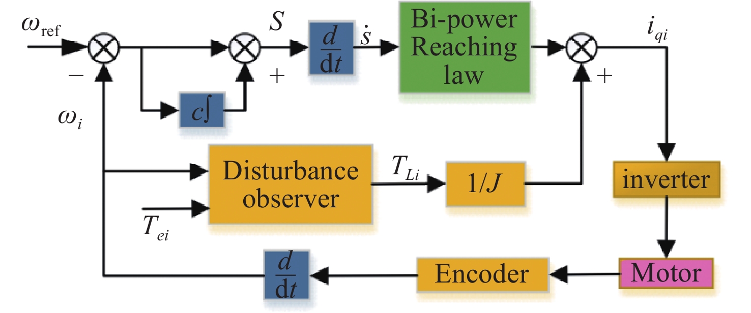
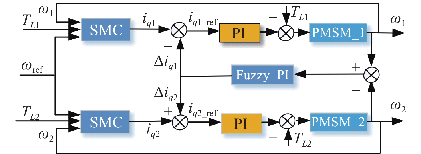
The block diagram of the final speed control law is shown in Fig. 1.

图 1.

Fig. 1. Block diagram of the speed controller

下载图片 查看所有图片

4 Design of the load-based torque observer

Generally, the load torque and external disturbance torque in the PMSM control system are regarded as the total torque. The reasonable design of the observer can effectively observe the load torque and calculate the motor current in equation (34) to realize disturbance suppression of the system. The total torque can be regarded as a constant value within a control period, which means

$ \frac{{\rm{d}}{T}_{Li}}{{\rm{d}}t}=0\quad. $ (35)

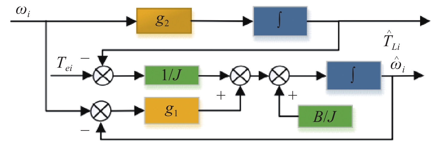
In order to obtain the estimated value of the total torque T_Li, the disturbance observer can be designed according to modern control theory and the gain in the observer can be reasonably configured to observe the rotational speed and the total disturbance torque. The state equation of the system is constructed as follows

$ \left\{\begin{array}{c}\dot{{\boldsymbol{x}}}={\boldsymbol{Ax}}+{\boldsymbol{Bu}}\\ {\boldsymbol{y}}={\boldsymbol{Cx}}+{\boldsymbol{Du}}\end{array}\right. \quad,$ (36)

in a nonlinear time-varying feedback system, where

$ {\boldsymbol{A}}=\left[\begin{array}{cc}-\dfrac{{B}_{i}}{{J}_{i}}& -\dfrac{1}{{J}_{i}}\\ 0& 0\end{array}\right],{\boldsymbol{B}}=\left[\begin{array}{c}\dfrac{1}{{J}_{i}}\\ 0\end{array}\right],{\boldsymbol{C}}=\left[\begin{array}{cc}1& 0\end{array}\right]\quad, $ ()

$ {\boldsymbol{D}} = \left[\begin{array}{cc}0\\ 0\end{array}\right] , {\boldsymbol{x}} = \left[\begin{array}{cc}\omega_i\\ T_i\end{array}\right] , {\boldsymbol{y}} = \omega_i , u = T_{ei}\quad. $ ()

We can know

$ {\rm{rank}}\left[\begin{array}{c}{\boldsymbol{C}}\\ {\boldsymbol{CA}}\end{array}\right]={\rm{rank}}\left[\begin{array}{cc}1& 0\\ -\dfrac{{B}_{i}}{{J}_{i}}& -\dfrac{1}{{J}_{i}}\end{array}\right]=2 \quad.$ ()

It can be seen that the system is fully observable. The observer and observation error equations are constructed as follows

$ \left\{\begin{array}{c}\dot{\widehat{{\boldsymbol{x}}}}={\boldsymbol{A}}\widehat{{\boldsymbol{x}}}+{\boldsymbol{B}}u+{\boldsymbol{G}}\left({\boldsymbol{y}}-\widehat{{\boldsymbol{y}}}\,\right)\\ \dot{{\boldsymbol{e}}}=\dot{{\boldsymbol{x}}}-\dot{\widehat{{\boldsymbol{x}}}}=\left({\boldsymbol{A}}-{\boldsymbol{GC}}\right){\boldsymbol{e}}\end{array}\right.\quad. $ (37)

The matrix G = $ \left[\begin{array}{c}g_1\\ g_2\end{array}\right] $can be found so that the eigenvalues of the matrix (A−GC) are located in the left half-plane by the pole configuration. The observation error e between the observed $\hat T_L $ and the actual T_L can be close to zero in finite time. Fig. 2 is the block diagram of the total disturbance torque observer.

图 2.

Fig. 2. Structural block diagram of the disturbance torque observer

下载图片 查看所有图片

5 Speed synchronization controller design

The cross-coupling control adopts speed synchronization error compensation current to make the double-PMSM respond quickly and realize speed synchronization. However, the speed error synchronization coefficient in cross-coupling control is usually difficult to obtain through theoretical analysis. Therefore, a cross-coupling synchronization control algorithm based on an improved double-power sliding mode control and fuzzy adaptive PI control is designed to improve the system’s accuracy.

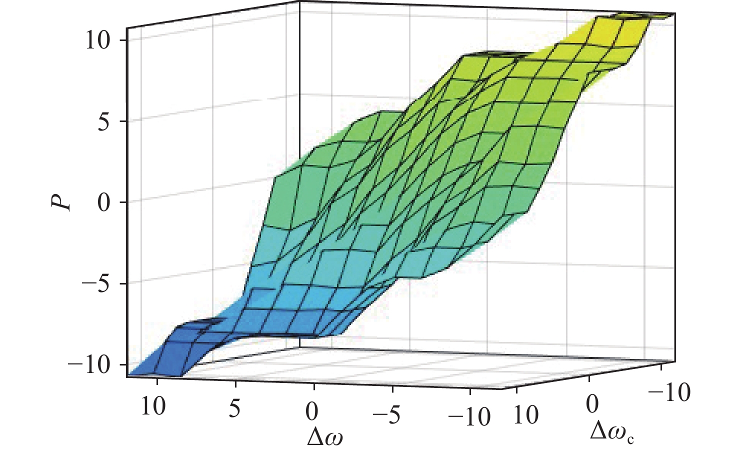
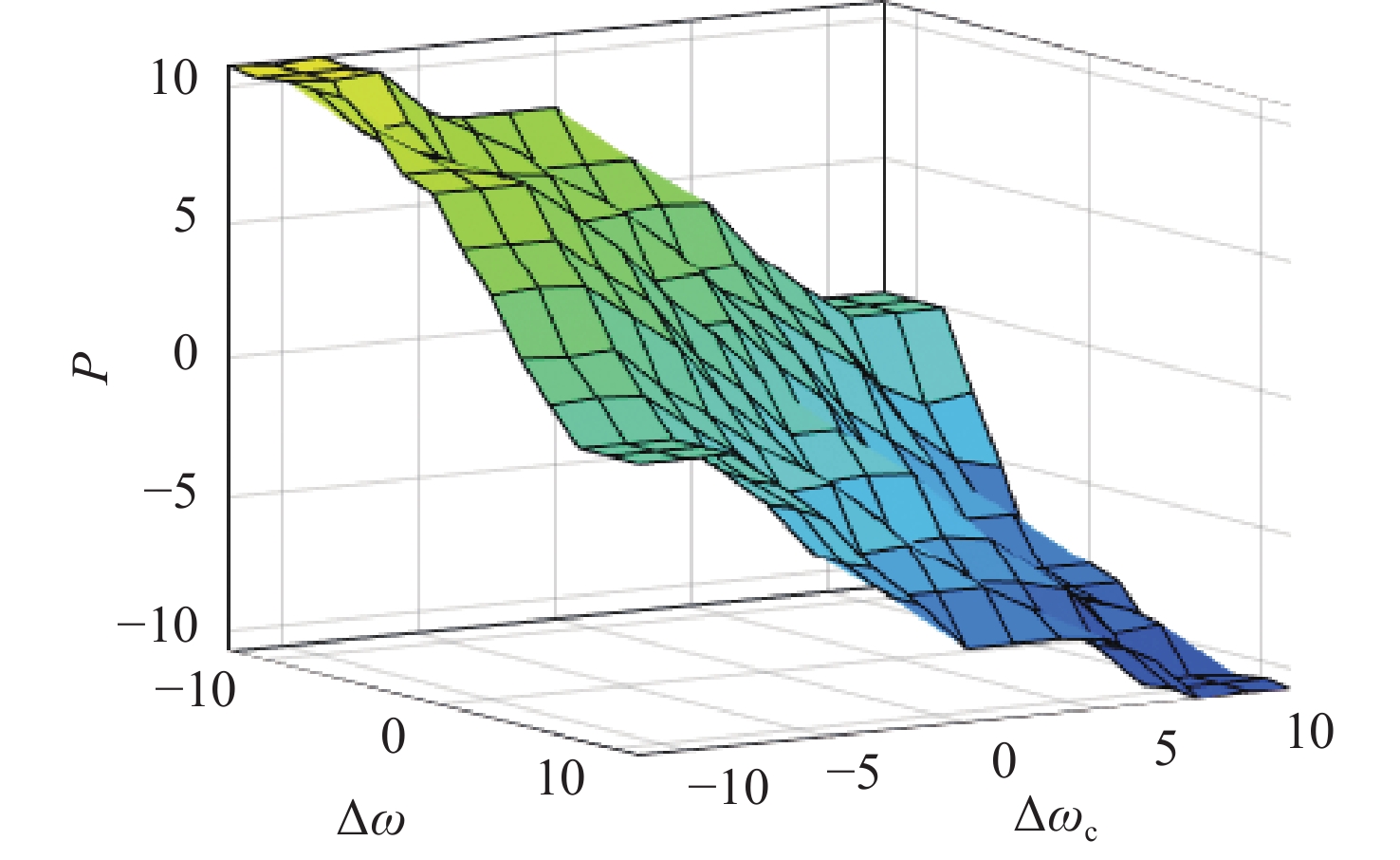
For the fuzzy adaptive PI control, the synchronization errors ∆ $\omega $ and its rate of change ∆ $\omega $ are the input and the current compensation is the output (Define ∆ $\omega={\omega_1}-{\omega_2} $, ∆ $\omega_c $=∆ $\omega $/∆t). The k_p and k_i values of the PI controller are continuously adjusted through ∆k_p and ∆k_i online. When e is large, a large k_p and k_i should be taken to reduce the error. When e is moderate, a moderate k_p and k_i should be moderated to avoid overshoot of the synchronous system. When e is small, a small k_p and k_i should be selected to avoid the impact of the synchronous system and give adaptive adjustment ability. Table 1 and Table 2 are the fuzzy rules of k_p and k_i. Figs. 3-4 (color online) show the relationship of the surface of ∆k_p and ∆k_i . The control diagram of the Dual-PMSMs synchronous system is shown in Fig. 5.

图 3.

Fig. 3. Surface diagram of ∆k_p value output

下载图片 查看所有图片

图 4.

Fig. 4. Surface diagram of ∆k_i value output

下载图片 查看所有图片

图 5.

Fig. 5. Overall block diagram of dual-motor synchronous control system

下载图片 查看所有图片

6 Simulation and analysis

The purpose of the current study is to determine the speed synchronization performance and anti-interference of a Dual-PMSM system. In order to verify the performance of the proposed control strategy, a Dual-PMSMs synchronous control modeling simulation is performed in MATLAB/Simulink. The parameters of Dual-PMSMs and the controller parameters are shown in Tables 3 and 4. The simulated speed response waveform of the proposed improved bi-power reaching method and traditional reaching method is compared in Fig.6 (color online) with reference speeds from 800 r/min to 1200 r/min. It can be seen that the improved bi-power reaching method control has less adjustment time (Traditional reaching method speed controller parameter: k=30; The improved bi-power reaching method speed controller parameters are shown in Table 4 PMSM1.).

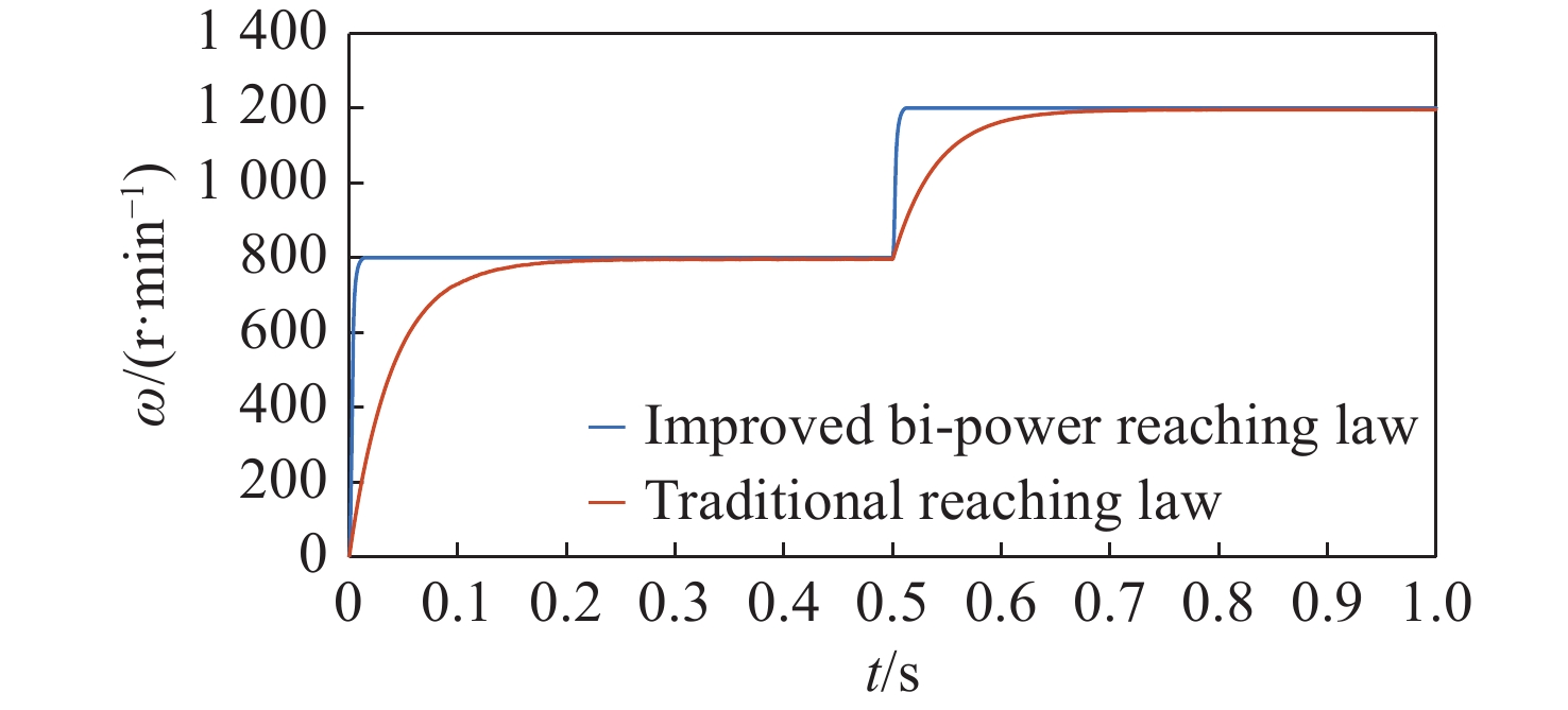
图 6.

Fig. 6. Comparison of speed response waveforms between the improved and traditional reaching methods

下载图片 查看所有图片

It can be seen that the parameters of the two motors is different and the process is more difficult than it is for motors with the same parameters. The parameters of the current loop PI controller are the same between the two control strategies, where k_p = 350 and k_p = 82 500. The speed PI controller parameters of the traditional double PI parallel cross-coupling control method are designed at k_p = 0.02 and k_i = 1.

The performance comparison between the traditional double PI cross-coupling control from no-load torque and sudden load torque perturbation is shown in Figs. 7-Fig. 10 when the reference speed is ω_ref = 800 r/min.

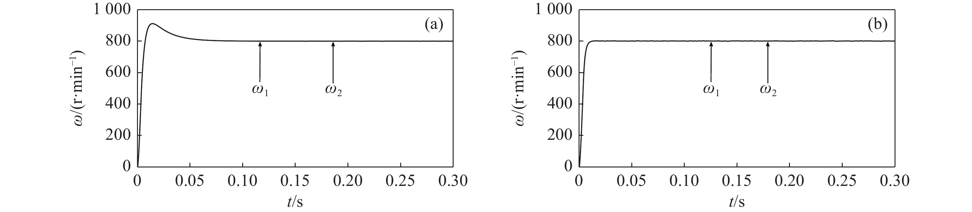
图 7.

Fig. 7. Speed waveforms obtained by different methods under no-load torque starting condition. (a) Conventional cross-coupled control. (b) Improved bi-power reaching method

下载图片 查看所有图片

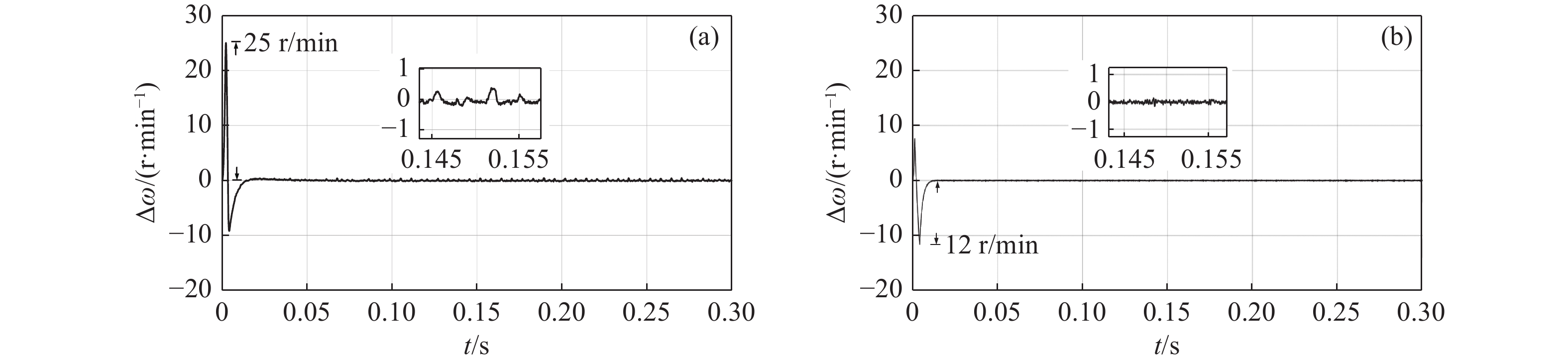
图 8.

Fig. 8. Synchronization error waveforms obtained by different methods under no-load torque startup condition. (a) Conventional cross-coupling control. (b) Improved bi-power reaching method sliding mode control

下载图片 查看所有图片

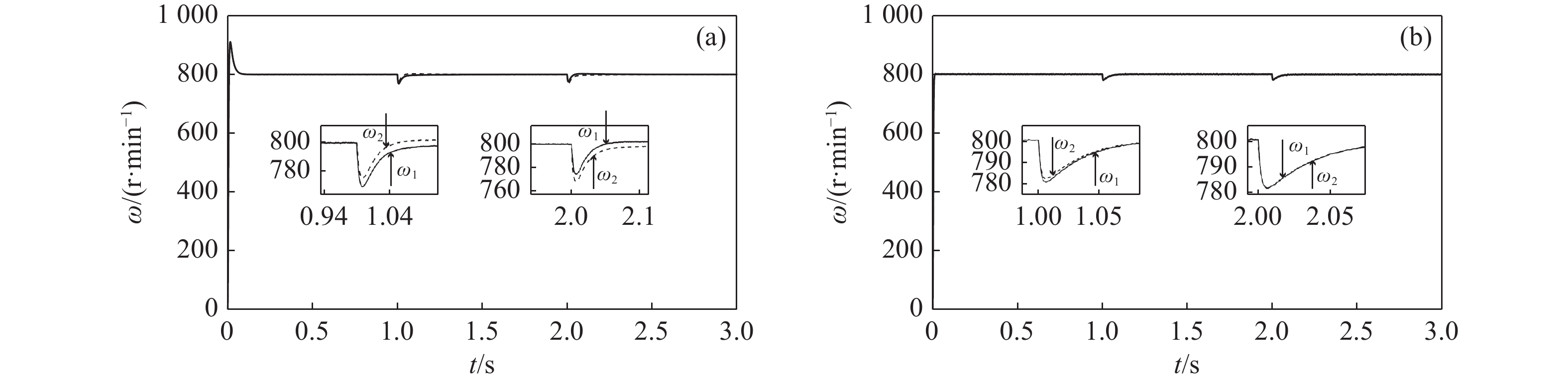
图 9.

Fig. 9. Torque speed waveforms obtained by different methods under sudden load torque condition. (a) Conventional cross-coupling control. (b) Improved bi-power reaching method sliding mode control

下载图片 查看所有图片

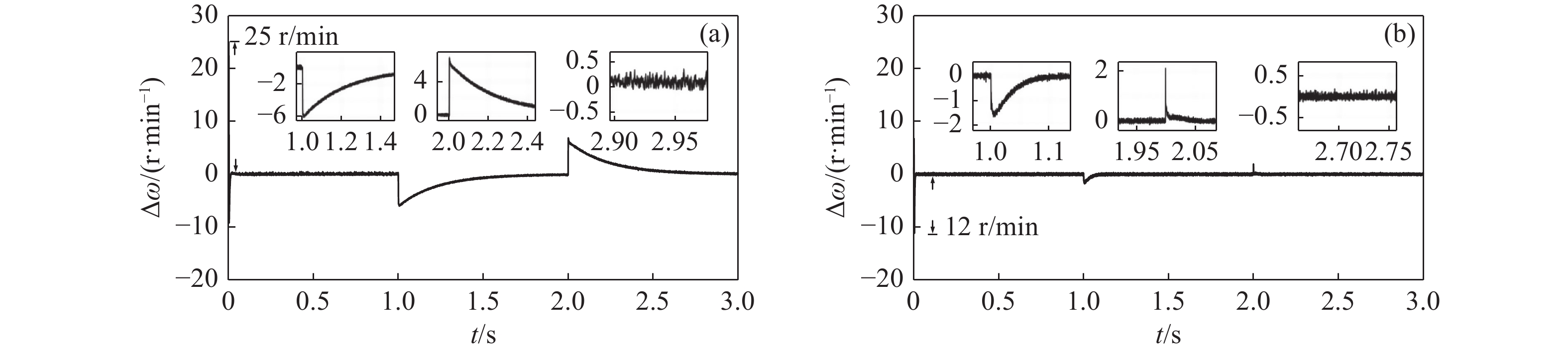
图 10.

Fig. 10. Synchronization error waveforms obtained by different methods under sudden surge load torque condition. (a) Conventional cross-coupling control. (b) Improved bi-power reaching method sliding mode control

下载图片 查看所有图片

From Fig. 7(a), it can be seen that traditional dual PI parallel cross-coupling control has a larger overshoot at no-load torque start and it reaches the reference speed after 0.075 s. The designed control strategy in this paper has no overshoot and can reach the reference speed in 0.015 s, as shown in Fig. 7(b). Due to the different parameters of the two motors, the speed synchronization error of the Dual-PMSMs is larger whether uses the traditional cross-coupling control strategy or the improved bi-power reaching sliding mode control method at startup. From Fig. 8(a) we can know that the maximum synchronization error can reach 25 r/min at the reference speed of 800 r/min when use the traditional cross-coupling control strategy. However, Fig. 8(b) shows that the maximum speed error of the proposed control strategy is 12 r/min under no-load torque startup conditions.

The speed waveform and the synchronization error waveform are shown in Fig. 9, where a 2 N·m load torque is suddenly applied to motor 1 at 1 s and a 2.5 N·m load torque is suddenly applied to motor 2 at 2 s. Fig. 10(a) shows that the large synchronization error is 7 r/min with sudden load torque and it can reach stability after 0.2 s under the conventional cross-coupling controller. Fig. 10 (b) shows that the proposed control strategy has a maximum speed synchronization error of 2.2 r/min with sudden load torque and reaches stability after 0.1 s (Fig. 10). Thus, the improved method has better anti-disturbance performance and speed tracking capabilities than those of the traditional control algorithm.

7 Conclusion

Based on the traditional cross-coupling control, an integral sliding mode speed tracking controller based on bi-power reaching method is designed and an observer is introduced into the sliding mode control rate to enhance the robustness and anti-disturbance of the system. A speed synchronization controller based on fuzzy adaptive PI control adjusts the PI parameters of the speed synchronous controller according to the real-time synchronization error. The comparison experimetal indicates that the system has certain adaptive adjustment ability for external disturbance.