1 Introduction

The 3D measurement technology based on structured light has the advantages of non-contact, high efficiency, and low cost, which is widely used in industrial measurement, mold manufacturing, medical image, cultural relic reconstruction and other fields^[1-4]. The 3D measurement technology based on phase-shift and fringe projection has good measurement accuracy, density, and anti-interference ability, and is most widely used in high-precision static measurement^[5]. However, in the dynamic 3D measurement, the movement of the object changes the ideal correspondence between the object points, image points, and phases in different fringe images. Under this condition, the application of traditional phase formulas will produce significant phase measurement errors, which will greatly reduce the accuracy of the 3D measurement.

For the dynamic 3D measurement, most researches tend to use single-frame structured light projection technology^[6-8], but the inherent shortcomings of this technology in terms of measurement accuracy and anti-interference ability cannot be ignored. Some researches apply high-speed photography technology to reduce the time interval of different fringe images, so as to suppress the dynamic 3D measurement errors^[9-12]. This technology is mainly suitable for the situation where the object movement speed is low, and the measurement accuracy is not high. LIU Y J^[13] and WEISE T^[14] propose the dynamic 3D measurement error compensation technology based on phase-shifting and fringe projection, which accurately restores the phase by analyzing the equivalent phase-shifting errors. The process of this technology is generally as follows. First, the phase distribution of each image and the phase-shifting between different images are calculated by the Fourier assisted phase-shifting method^[15-16]. Second, the phase distribution of the moving object is calculated by using the equal-step phase-shifting method or the random step-size phase-shifting algorithm based on least squares^[17-18]. The main problem of this technology is that the phase-shifting between different images calculated by Fourier assisted phase-shifting method has not enough precision. In fact, there is no essential difference between the phase calculation accuracy of this technology and that of the single-frame structured light projection technology.

A new dynamic 3D measurement error compensation technology based on phase-shifting and fringe projection is proposed in this paper. Fristly, by using the improved Fourier assisted phase shift method and the improved iterative algorithm based on the least square method, the calculation accuracy of the phase-shifting between different images is improved, and then the calculation accuracy of the phase of moving object is improved. In the process, the improved Fourier assisted phase-shifting method introduces a double elliptical filter window, which not only fully retains the spectrum information, but also greatly reduces the influence of redundant noise data, effectively suppresses the error diffusion of mutation position, and improves the accuracy of phase shift analysis. The advanced iterative algorithm based on least squares^[19] takes the equivalent phase-shifting obtained by the improved Fourier assisted phase-shifting method as the initial value, and uses the random step-size phase-shifting algorithm to iteratively calculate the equivalent phase shift and phase until the accuracy meets the requirements. For the mature technologies in static 3D measurement, such as calibration technology^[20-24] and phase unwrapping technology^[25-26], will not be discussed in detail in this paper.

2 Principle

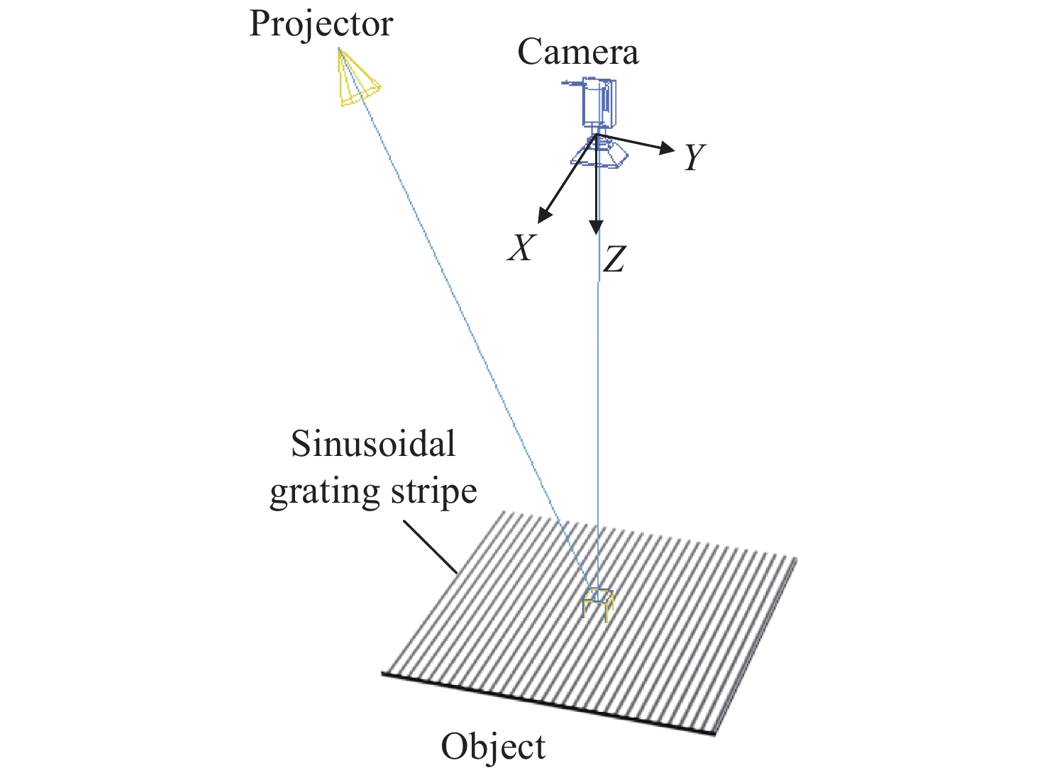
The 3D measurement system based on phase-shifting and fringe projection is shown in Fig. 1. The basic principle of the dynamic 3D measurement errors is introduced by taking the three-step phase-shifting method as an example.

图 1.

Fig. 1. The 3D measurement system based on phase-shifting and fringe projection

下载图片 查看所有图片

For a static object, the pixel coordinates of a point on the object in different images are the same, and the image grayscales of this point are as follows:

$ \left\{\begin{split} &{I}_{1}(x,y)={I}_{d}+{I}_{e}.\mathrm{cos}\left(\varphi (x,y)-2\mathrm{{\text{π}} }/3\right)\\ &{I}_{2}(x,y)={I}_{d}+{I}_{e}.\mathrm{cos}\left(\varphi (x,y)\right)\\ &{I}_{3}(x,y)={I}_{d}+{I}_{e}.\mathrm{cos}\left(\varphi (x,y)+2\mathrm{{\text{π}} }/3\right) \end{split}\right.\quad, $ (1)

in the formula, I_d andI_e represent the background intensity and modulation intensity, respectively, and $ \varphi (x,y) $ represents the initial phase of the fringe images. According to the three-step phase-shifting method, the phase formula is as follows:

$ \varphi (x,y)={\rm{arctan}}\left(\sqrt{3}\times \frac{{I}_{1}\left(x,y\right)-{I}_{3}\left(x,y\right)}{{2I}_{2}\left(x,y\right)-{I}_{1}\left(x,y\right)-{I}_{3}\left(x,y\right)}\right) .$ (2)

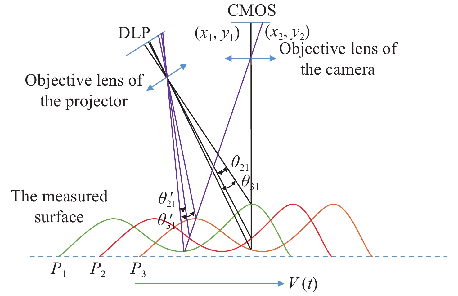
For a moving object, the basic principle of the dynamic 3D measurement errors can be analyzed through reverse thinking, as shown in Fig. 2. If the object moves along the $ V\left(t\right) $ direction, the phase of fringe images changes along this direction, and the object is located at P₁, P₂, and P₃ at different shooting times. In different fringe images, the image grayscales at $ (x_1,y_1) $ are as follows:

图 2.

Fig. 2. The equivalent phase-shifting errors of the same pixel coordinate position

下载图片 查看所有图片

$ \left\{\begin{split} &{I}_{1}(x_1,y_1)={I}_{d}+{I}_{e}.{\rm{cos}}\left(\varphi (x_1,y_1)-\frac{2{\text{π}} }{3}\right)\\ &{I}_{2}(x_1,y_1)={I}_{d}+{I}_{e}.{\rm{cos}}\left(\varphi (x_1,y_1)-{\theta }_{21}(x_1,y_1)\right)\\ &{I}_{3}(x_1,y_1)={I}_{d}+{I}_{e}.{\rm{cos}}\left(\varphi (x_1,y_1)+\frac{2{\text{π}} }{3}-{\theta }_{31}(x_1,y_1)\right) \end{split} \right.. $ (3)

At this time, there will be significant errors in calculating the phase of this position by using formula (2). Although the errors are caused by the movement of the object, they can be equivalent to the phase-shifting errors of $ {\theta }_{21}(x_1,y_1) $ and $ {\theta }_{31}(x_1,y_1) $. In the same way, there are equivalent phase-shifting errors of $ {\theta }_{21}^{\mathrm{\text{'}}}(x_2,y_2) $ and ${\theta }_{31}'(x_2,y_2)$ at $ (x_2,y_2) $. Normally, the equivalent phase-shifting errors are not equal step, that is ${\theta }_{31}(x_1,y_1)\ne {2\times \theta }_{21}(x_1,y_1)$, ${\theta }_{31}'(x_2,y_2)\ne {2\times \theta }_{21}'(x_2,y_2)$. The equivalent phase-shifting errors of different pixel positions are also different, that is ${\theta }_{21}(x_1,y_1)\ne {\theta }_{21}'(x_2,y_2)$, ${\theta }_{31}(x_1,y_1)\ne {\theta }_{31}'(x_2,y_2)$.

If the equivalent phase shift between different images can be accurately analyzed, the dynamic 3D measurement error will be effectively suppressed and the dynamic 3D measurement accuracy will be improved.

3 Methods

3.1 The improved Fourier assisted phase-shifting method

The Fourier-assisted phase-shifting method is a global analysis method. At the locations of fringe mutation, the phases calculated by this method have large errors, and the errors will spread around the locations of fringe mutation in the form of gradual attenuation fluctuations. A window function is added to the Fourier transform process to effectively limit the spread of the errors, which helps to improve the calculation accuracy of the global phases. The windowed Fourier transform is as follow:

$\begin{split} F\left(u,v\right)=&\frac{1}{M\times N}\times \sum _{x=1}^{M}\sum _{y=1}^{N}I\left(x,y\right)\times\\ &W(x-{x}_{0},y-{y}_{0}){{\rm{e}}}^{-{\rm{j}}2{\text{π}} \left(\tfrac{ux}{M}+\tfrac{vy}{N}\right)}\quad. \end{split} $ (4)

In the formula, $ I\left(x,y\right) $ represents the gray distribution of the fringe image, $ W(x-{x}_{0},y-{y}_{0}) $ is the window function, $ {x}_{0} $ and $ {y}_{0} $ represent the center pixel coordinates of the window function; M and N are the number of pixels in two directions. The Gaussian function is chosen as the window function, and the function is as follow:

$ W(x-{x}_{0},y-{y}_{0})=\frac{1}{\sqrt{2{\text{π}} }\delta }\exp\left(-\frac{{\left(x-{x}_{0}\right)}^{2}+{\left(y-{y}_{0}\right)}^{2}}{2{\delta }^{2}}\right) ,$ (5)

in the formula, $ \delta $ is the standard deviation of the normal distribution, which can be used to adjust the size of the window and the smoothing effect of the filter. The larger the $ \delta $, the larger the window, the better the smoothing effect of the filter.

The spectrum distribution in the window field centered on $ ({x}_{0},{y}_{0}) $ can be obtained through formula (4) and formula (5). Then, it is necessary to select an appropriate band-pass filter to filter the spectrum information other than the first-order spectrum and extract the fundamental frequency spectrum containing object height information. The mathematical expression of frequency domain filtering is as follow:

$ G\left(u,v\right)=H\left(u,v\right)F\left(u,v\right)\quad, $ (6)

in the formula, $ F\left(u,v\right) $ is the spectrum distribution obtained by the windowed Fourier transform, $ H\left(u,v\right) $ is the frequency domain filter, and $ G\left(u,v\right) $ is the filtered spectrum distribution.

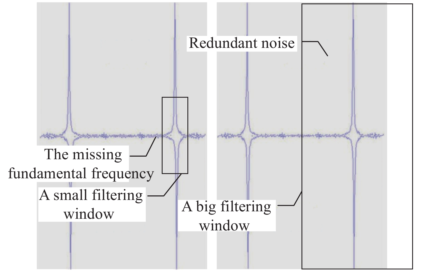
The traditional frequency domain filter uses a rectangular window, as shown in Fig. 3. This type of filter cannot completely extract all the first-order spectrum. Moreover, it retains a large amount of redundant noise data in the extraction area, which affects the analysis accuracy of spectrum distribution. The Gaussian window filter can improve the above problems to a certain extent, but the design of the window shape is still not flexible enough. The existed research shows that the first-order spectrum usually presents an elliptical distribution^[27], so a two-way elliptical filter is proposed in this paper, as shown in Fig. 4.

图 3.

Fig. 3. Rectangular window filter

下载图片 查看所有图片

图 4.

Fig. 4. Double elliptical window filter

下载图片 查看所有图片

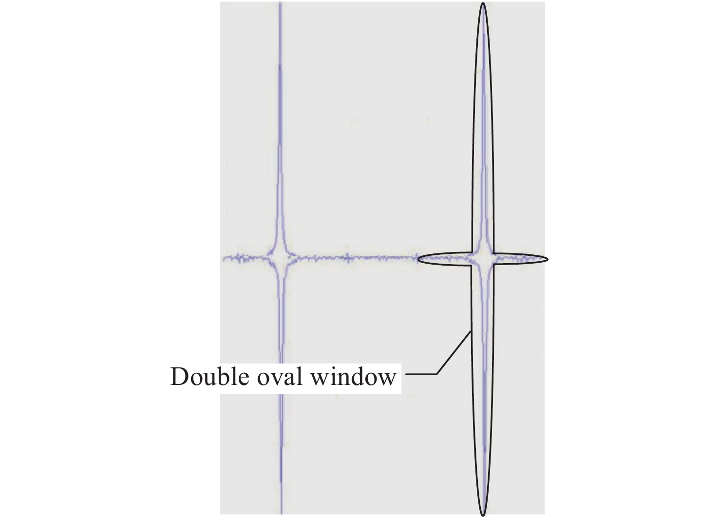
The mathematical expression of the double ellipse filter is as follow:

$ H\left(u,v\right)=\left\{ \begin{split} &1\quad\frac{{(u-{u}_{0})}^{2}}{{R}_{u1}^{2}}+\frac{{(v-{v}_{0})}^{2}}{{R}_{v1}^{2}}\leqslant 1\;{\rm{and}}\;\frac{{(u-{u}_{0})}^{2}}{{R}_{u2}^{2}}+\frac{{(v-{v}_{0})}^{2}}{{R}_{v2}^{2}}\leqslant 1\\ &0\quad{\rm{else}} \end{split}\right. \quad.$ (7)

In the formula, $ {u}_{0} $ and $ {v}_{0} $ represent the center coordinates of the filter window, they can be determined by local centroid algorithm. $ {R}_{u1} $, $ {R}_{v1} $, $ {R}_{u2} $ and $ {R}_{v2} $ represent the radius of the double ellipse in two directions, they are not strictly limited, in principle, the filter needs to contain complete first-order spectrum information and reduce redundant noise data as much as possible.

After the frequency domain filtering is completed, the remaining calculation steps are consistent with the traditional Fourier assisted phase-shifting method. Perform inverse Fourier transform on the extracted fundamental frequency to obtain spatial information, and the phase at different positions can be obtained by moving the Gaussian window. The phase difference of the two fringe images can be used to obtain the phase-shifting of the position.

3.2 The advanced iterative algorithm based on least squares

The process of the advanced iterative algorithm based on least squares is shown in Fig. 5.

图 5.

Fig. 5. The process of the advanced iterative algorithm based on least squares

下载图片 查看所有图片

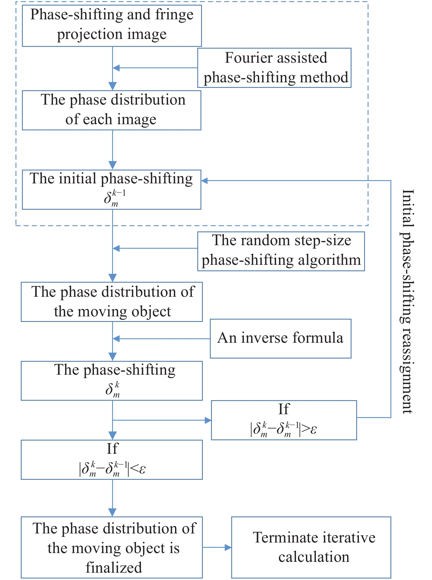
In Fig. 5, $ {\delta }_{m} $ is the phase-shifting distribution of the fringe image m, $m=1,2,3,\cdots,M(M\geqslant 3)$. K is the number of iterations, and ε is the convergence threshold set according to the accuracy.

The initial phase-shifting can be preliminarily calculated by the improved Fourier assisted phase-shifting method. Generally, the phase-shifting is random and unequal-step. In this case, the phase needs to be calculated by the random step-size phase-shifting algorithm based on least squares. The formulas are as follows:

$ {\boldsymbol{A}}=\left[\begin{array}{ccc}M& \displaystyle\sum _{m=1}^{M}\cos{\delta }_{m}(x,y)& \displaystyle\sum _{m=1}^{M}\sin{\delta }_{m}(x,y)\\ \displaystyle\sum _{m=1}^{M}\cos{\delta }_{m}(x,y)& \displaystyle\sum _{m=1}^{M}{\cos}^{2}{\delta }_{m}(x,y)& \displaystyle\sum _{m=1}^{M}\cos{\delta }_{m}(x,y)\sin{\delta }_{m}(x,y)\\ \displaystyle\sum _{m=1}^{M}\sin{\delta }_{m}(x,y)& \displaystyle\sum _{m=1}^{M}\sin{\delta }_{m}(x,y)\cos{\delta }_{m}(x,y)& \displaystyle\sum _{m=1}^{M}{\sin}^{2}{\delta }_{m}(x,y)\end{array}\right] $ (8)

$ {\boldsymbol{B}}={\left[\begin{array}{ccc}\displaystyle\sum _{m=1}^{M}{I}_{m}'\left(x,y\right)& \displaystyle\sum _{m=1}^{M}{I}_{m}'\left(x,y\right)\cos{\delta }_{m}(x,y)& \displaystyle\sum _{m=1}^{M}{I}_{m}'\left(x,y\right)\sin{\delta }_{m}(x,y)\end{array}\right]}^{{\rm{T}}} \quad,$ (9)

$ \left\{{\boldsymbol{X}}\right\}={\left[{\boldsymbol{A}}\right]}^{-1}\left[{\boldsymbol{B}}\right]={\left[\begin{array}{ccc}a& b& c\end{array}\right]}^{{\rm{T}}} \quad,$ (10)

$ \varphi (x,y)=-{\rm{arctan}}\frac{c}{b} \quad.$ (11)

In the formulas, M is the number of the projected fringe image, $ {\delta }_{m}(x,y) $ is the phase-shifting distribution of the fringe image m, and $ {I}_{m}^{\mathrm{\text{'}}}\left(x,y\right) $ is the gray distribution of m collected by camera.

In the high-precision dynamic 3D measurements, the accuracy of the phase-shift calculated by the improved Fourier assisted phase-shifting method cannot always meet the requirement. Therefore, the advanced iterative algorithm based on least squares is proposed in this paper, which can calculate the phase-shifting and phase more accurately. The basic ideas of the advanced iterative algorithm based on least square are as follows. First, the phase-shifting calculated by the improved Fourier assisted phase-shifting method is taken as the initial value, and the phase distribution is calculated, where $ m=1,2,3,\cdots,M(M\geqslant 3) $. Then, the phase-shifting is recalculated by using the phase distribution. After several iterations, the convergence condition is satisfied. The convergence condition is as follow:

$ \left|{\delta }_{m}^{k}-{\delta }_{m}^{k-1}\right| < \varepsilon \quad,$ (12)

In the iterative process, a method for calculating the phase-shifting with known phase distribution is proposed. The method is based on the principle of least square, and its objective function is designed as follows:

$ \begin{split} &{S}\left(x,y\right)=\sum _{m=1}^{M}{\left({I}_{m}\left(x,y\right)-{I}_{m}'\left(x,y\right)\right)}^{2} =\\ &\sum _{m=1}^{M}{\left({a}_{m}+{b}_{m}\cos\varphi \left(x,y\right)+{c}_{m}\sin\varphi \left(x,y\right)-{I}_{m}'\left(x,y\right)\right)}^{2}\quad, \end{split} $ (13)

in the formula, $ {I}_{m}\left(x,y\right) $ is the theoretical gray distribution of the fringe image m. $ {a}_{m}={I}_{d} $, ${b}_{m}= {I}_{e}\cos{\delta }_{m}(x,y)$, ${c}_{m}= {-I}_{e}\sin{\delta }_{m}(x,y)$. I_d and I_e represent the background intensity and modulation intensity, respectively, and $ {\delta }_{m}(x,y) $ is the phase-shifting distribution of the fringe image m.

To minimize $ S\left(x,y\right) $, let $ \partial S\left(x,y\right)/\partial {a}_{m} $ = 0, $ \partial S\left(x,y\right)/\partial {b}_{m} $ = 0, $ \partial S\left(x,y\right)/\partial {c}_{m} $ = 0, where $m=1,2, 3,\cdots,M(M\geqslant 3)$, and the following formulas can be obtained:

$ {\boldsymbol{A}}=\left[\begin{array}{ccc}1& \cos\varphi \left(x,y\right)& \sin\varphi \left(x,y\right)\\ \cos\varphi \left(x,y\right)& {\cos}^{2}\varphi \left(x,y\right)& \cos\varphi \left(x,y\right)\sin\varphi \left(x,y\right)\\ \sin\varphi \left(x,y\right)& \cos\varphi \left(x,y\right)\sin\varphi \left(x,y\right)& {\sin}^{2}\varphi \left(x,y\right)\end{array}\right]\quad, $ (14)

$ {\boldsymbol{B}}={\left[\begin{array}{ccc}{I}_{m}'\left(x,y\right)& {I}_{m}'\left(x,y\right)\cos\varphi \left(x,y\right)& {I}_{m}'\left(x,y\right)\sin\varphi \left(x,y\right)\end{array}\right]}^{{\rm{T}}}\quad, $ (15)

$ \left\{{\boldsymbol{X}}\right\}={\left[{\boldsymbol{A}}\right]}^{-1}\left[{\boldsymbol{B}}\right]={\left[\begin{array}{ccc}{a}_{m}& {b}_{m}& {c}_{m}\end{array}\right]}^{{\rm{T}}}\quad, $ (16)

$ {\delta }_{m}(x,y)=-{\rm{arctan}}\frac{{c}_{m}}{{b}_{m}} \quad.$ (17)

4 Experimental verification

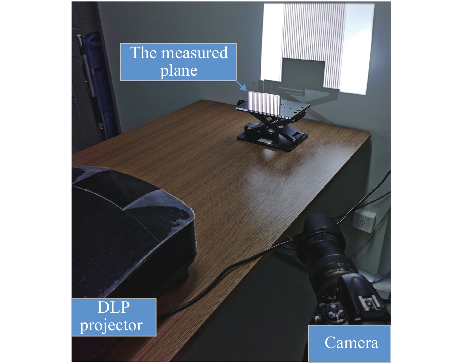
To verify the theory and method, a dynamic 3D measurement system based on phase-shift and fringe projection was established. The measurement system consists of a camera, a projector, and a measured object. The camera is a Nikon d850 SLR, the focal length of its objective lens is 35 mm, and the camera had a CMOS size of 24 mm × 16 mm (DX mode) and a resolution of 2704 × 1800. The projector is Benq W7000 DLP with a resolution of 1920 × 1080. The projection was encoded as a four-step phase-shift fringe, and the period of the phase-shift takes up 32 DLP pixels. The angle between the optical axis of the camera objective and the projection objective was about 15°. The distance between the photographic center and the measured object was about 1500 mm, and the pixel resolution of the camera is about 0.35 mm.

An object with a moving speed of about 100 mm/s was originally planned to be measured. The projector and the camera are connected through a synchronous trigger to implement time match of the projection and imaging. The integration time of single imaging of the camera can be set as 1/1000 s, the time interval between two adjacent projections and imaging is set as 1s. However, to reduce the cost of the experiment, we moved the measured object three times along the direction of gray scale change, and then projected and took pictures of the object in three static states, which equivalently replaces the measurement process of moving object. The biggest difference between this alternative and the actual situation is that it is difficult to simulate the image blur caused by object motion in a single imaging time. However, in our envisaged measurement condition, the moving distance of the object in a single imaging time is only 0.1 mm, accounting for about 0.28 pixels in the image, so the dynamic blur of the image can be ignored.

In order to verify the accuracy of the method, a precision machined object is needed as the measurement benchmark. Because the machining accuracy of the flat plate is the easiest to achieve, a precision grinding aluminum plate with a size of 150 mm × 100 mm × 10 mm and a surface flatness better than 0.01mm is selected as the test object. In order to simulate the dynamic three-dimensional measurement of complex objects, the flat plate is deliberately placed obliquely along the optical axis of the camera, so that the depth distance of each point on the flat plate in the camera coordinate system is inconsistent. At this time, there is no great difference between measuring a flat plate and measuring a complex object, and the high accuracy of the flat plate is more conducive to the accuracy of our evaluation method.The measurement system is shown in Fig. 6.

图 6.

Fig. 6. The measurement system

下载图片 查看所有图片

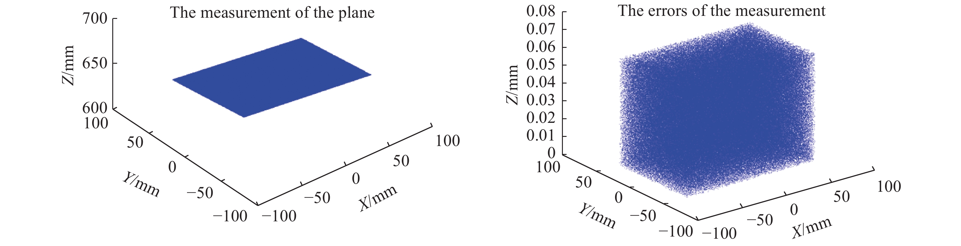
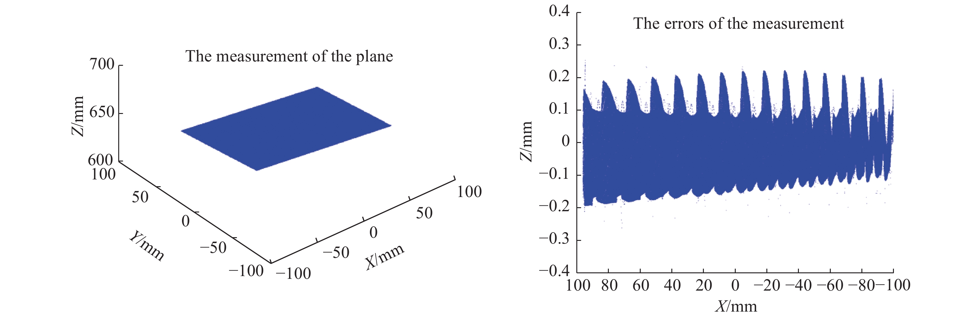
First, the 3D shape of the plane was measured in a static scene with a mean square error of 0.034 mm. The result is shown in Fig. 7.

图 7.

Fig. 7. The static measurement results

下载图片 查看所有图片

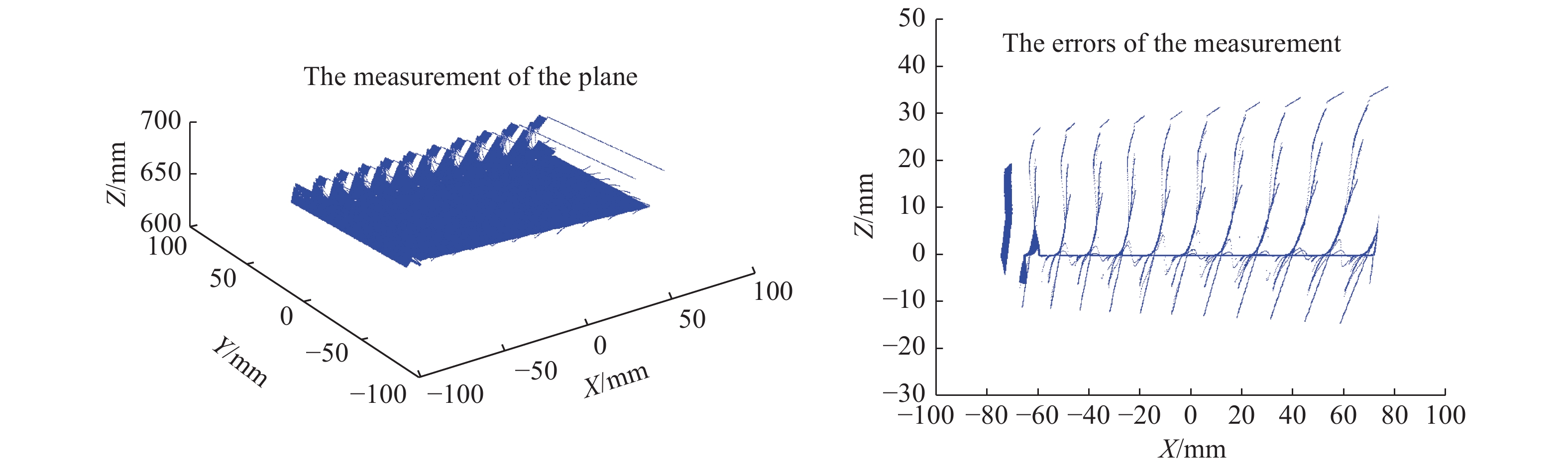
Then, the object was moved 4 mm, 5 mm and 6 mm in the direction of the gray scale change of the fringe. The mean square error of the uncompensated dynamic 3D measurement was 5.241 mm, as shown in Fig. 8.

图 8.

Fig. 8. The results of uncompensated dynamic 3D measurement

下载图片 查看所有图片

Finally, the dynamic 3D measurement error compensation technology proposed in this paper was used to measure again. The mean square error of the dynamic measurement was 0.132 mm, as shown in Fig. 9.

图 9.

Fig. 9. The results of compensated dynamic 3D measurement

下载图片 查看所有图片

The experimental results show that the dynamic 3D measurement error can be greatly reduced by using the error compensation technology proposed in this paper, and the accuracy of the dynamic 3D measurement can be better than 0.15 mm.

5 Conclusion

The basic principle of the dynamic 3D measurement errors is analyzed, and the dynamic 3D measurement error compensation method is proposed. This method combines the advanced iterative algorithm based on least squares and the improved Fourier assisted phase-shifting method to realize the high-precision calculation of random step-size phase-shifting and phase. The experimental results show that the dynamic 3D measurement error can be reduced by more than one order of magnitude by using the error compensation technology proposed in this paper, and the accuracy of the dynamic 3D measurement can be better than 0.15 mm.