Seeing through scattering media is highly desired in many occasions, such as remote sensing through clouds, fog, and haze; underwater detection; anti-terrorism surveillance; biological tissue imaging; and clinical diagnosis. However, multiple scattering experienced by photons when propagating in scattering media breaks the point-to-point correspondence required by traditional imaging methods^[1,2]. In order to solve the problem, people developed many techniques including time gating^{[35" target="_self" style="display: inline;">–5]}, wavefront shaping^{[6–10" target="_self" style="display: inline;">–10]}, diffuse optical tomography^[11], transmission matrix measurement^{[12–16" target="_self" style="display: inline;">–16]}, optical phase conjugation^{[17–23" target="_self" style="display: inline;">–23]}, speckle deconvolution^[24], and speckle autocorrelation^{[25–29" target="_self" style="display: inline;">–29]}. Among these methods, the speckle autocorrelation method exploits the memory effect (ME) to reconstruct the image of a hidden object from a speckle pattern, which is simple, fast, and non-invasive.

In speckle autocorrelation imaging, the autocorrelation of a speckle pattern consists of an autocorrelation of the object with a magnification factor determined by the experimental setup and a random noise background, which leads to a disturbed frequency spectrum of the object and sequentially a degraded reconstruction quality. This issue can be tackled by capturing a speckle pattern with a large sampling ratio R defined as R=rDurOv, where rD and rO are the radii of the detecting area and the object, respectively; for simplicity, only circular areas are considered here; and u and v are the distances from the object and the camera to the medium when it is thin, respectively. For an experimental setup with fixed values of u, rO, and rD, as R increases, more independent speckles are detected, resulting in a smoother noise background after ensemble averaging. Of course, the object is always within the ME range^[30] in the above discussion.

In experiment, for a small v, this condition can be easily satisfied by using an ordinary detector to capture a frame of speckles with a large R. However, in practice it is difficult to place the camera close to the media in some situations, which limits the sampling ratio and therefore the amount of valid information, resulting in a low-quality or even failed reconstruction. An intuitive solution is increasing the sensor area and/or employing a large aperture lens, however, this is expensive, space-consuming, and sometimes unrealistic.

In this Letter, by utilizing the equivalence between the spatial and temporal ensemble average of speckles^[2], we propose a simple and fast method for imaging through dynamic scattering media with a stitched speckle pattern. In particular, we acquire many speckle patterns with different point spread functions in sequence with a small sensor, stitch them together to get a big speckle pattern, and then reconstruct the image from the stitched pattern. In this way we can reconstruct the image well even when the sensor area is insufficient for a large image distance without any need for hardware upgrade. Compared to purely averaging (or summing) the autocorrelation, the stitching method can suppress the background noise and simultaneously increase the resolution of the power spectrum for more details, which is crucial in applications like remote sensing.

In the following, we first show the equivalence between the stitched speckle pattern and the one captured with a large camera sensor. Then we experimentally demonstrate the improvement of image quality with increased stitching number compared to pure averaging. Last, we perform simulations to study the trend of image quality with stitching number and the theoretical lower threshold of R for our method to be valid.

The ME is the prerequisite of speckle autocorrelation imaging, which essentially demonstrates that speckle patterns generated by different points within the ME range are shifted but highly correlated^[31,32]. When an object hidden behind the scattering medium (within the ME range) is illuminated by a spatially incoherent light source, the corresponding speckle pattern on the camera can be seen as a superposition of speckle patterns generated by all points of the object^[33]. In other words, the speckle pattern is a convolution of the object intensity and the point spread function (PSF), i.e., I(x,y)=O(x,y)*PSF(x,y),(1)where * denotes the convolution operator and O is the object intensity distribution. Then, the autocorrelation of the speckle pattern I can be expressed as $$\begin{gathered} I⋆I=(O*PSF)⋆(O*PSF) \\ =(O⋆O)*(PSF⋆PSF), \end{gathered}$$(2)where ⋆ is the correlation operator. For succinctness, the (x,y) coordinates are omitted here and afterward. Since the autocorrelation of the PSF is a peaked function^[25,27,33], Eq. (2) can be simplified as^[27]I⋆I≈O⋆O.(3)

According to the Wiener–Khinchin theorem, the power spectrum of an object is equal to the Fourier transform of its autocorrelation, |F(O)|2=F(O⋆O).(4)

Then we can reconstruct the image with a phase retrieval algorithm^[27,34,35].

Considering an imaging system with a detector of a large enough area, the PSF can be divided into n×m subblocks with the same size, each with its own PSFk, where k=1,2,3,…,n×m, as shown in Fig. 1(a). For simplicity, we choose m=n as follows. The autocorrelation of each PSFk is also a peaked function, and there is no mutual correlation between different subblocks. Similarly, the speckle pattern with a large sampling ratio can also be divided into n×n subblocks, each of which can be considered as the convolution of the object and the corresponding PSFk; that is, Ik=O*PSFk, where k=1,2,3,…,n×n, as shown in Fig. 1(b). The whole speckle pattern is seen as a combination of stitching these subblocks together, i.e., I=I1∪I2∪I3∪…∪In×n,(5)where ∪ is a stitching operator and n is defined as the stitching number. The autocorrelation of I turns to be $$\begin{gathered} I⋆I=∑k=1n×nIk⋆Ik+∑i=1n×n∑j=1n×nIi⋆Ij(i≠j) \\ ≈∑k=1n×nIk⋆Ik, \end{gathered}$$(6)where Ii⋆Ij(i≠j)≈0.

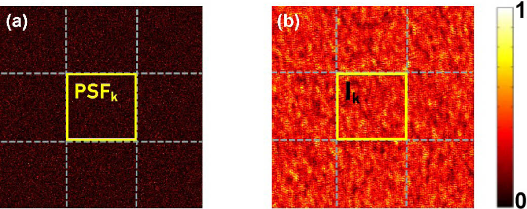
Fig. 1. Schematic illustration of stitching. (a) A big speckle pattern is split into many subblocks, and each subblock has its own independent PSFk. In other words, the big speckle pattern is obtained by stitching all independent subblocks together. (b) The segmentation of a big speckle pattern I.

下载图片 查看所有图片

For a dynamic scattering medium, here, only Brownian motion is considered, the PSF varies with time and the intensity fluctuation is ergodic in both spatial and temporal domains^[2], and the decorrelation time τ is used to quantify the decorrelation speed of the PSF. Assuming that we detect two PSFs, PSFt1 and PSFt2 at two different times t1 and t2; if t2−t1>τ, the two PSFs are independent. Referring to the stitching operation that uses different spatial subblocks mentioned above, we can acquire n×n independent frames of speckle patterns with different PSFs in sequence: Itk=O*PSFtk, k=1,2,3,…,n×n, and stitch them together into an n-by-n array to get a large speckle pattern I∪ (see Fig. 2) with an equivalent sampling ratio R∪=nR, I∪=It1∪It2∪It3∪…∪Itn×n.(7)

Fig. 2. Diagram of piecing together a series of speckle patterns {Itk}k=1n×n [shown as subfigure (a)] into (b) a big speckle pattern; the yellow square frame denotes a single speckle pattern Itk.

下载图片 查看所有图片

According to Eqs. (1)–(7), the Fourier transform amplitude of the object can be derived as |F(O)|=|F(I∪⋆I∪)|.(8)

Then the object can be reconstructed by an iterative phase-retrieval algorithm^[27]. This method increases the detection area digitally by stitching small speckle patterns together into a large one, and thus is especially suitable for the conditions with a small R. In addition, the stitching method differs from the autocorrelation averaging method in that the autocorrelation image of the former one has a greater number of pixels than the latter one, which thus leads to a finer Fourier spectrum. Specifically, if a single speckle pattern has N×N pixels, then its autocorrelation has 2N×2N pixels and the corresponding Fourier spectrum is a 2N×2N array. In stitching, the stitched pattern has an array size of nN×nN, resulting in a 2nN×2nN Fourier spectrum array. Hence, the spectral resolution accessible by the stitching method is n times that of the autocorrelation averaging method.

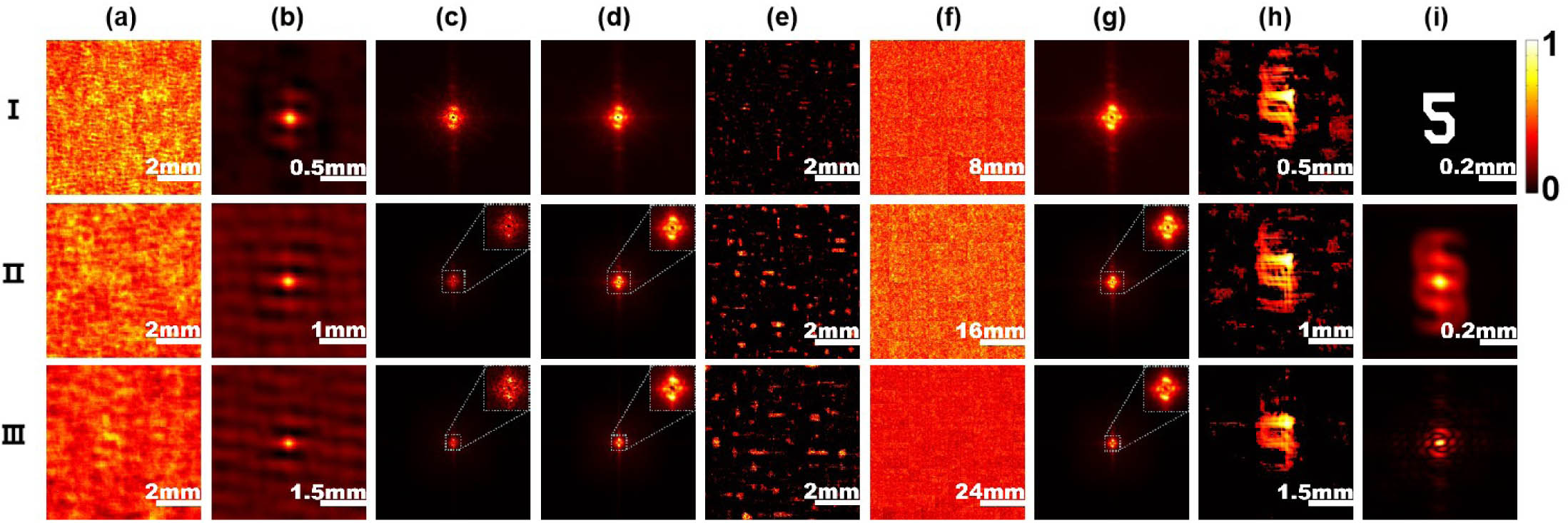
A schematic experimental setup is shown in Fig. 3. A pseudo thermal source generated by a 532 nm laser shining on a rotating ground glass disk illuminates a homemade binary object. The light emitted from the object transmits through a scattering layer and is detected by a CCD camera (AVT Stinggray F-504B) with an array size of 2452×2056 and a pixel pitch of 3.45μm. An iris with a diameter of 3mm is placed close to the exit surface of the layer to control the contrast and size of the recorded speckles. The scattering layer is made of tissue-mimicking porcine gelatin (a mixture of porcine gelatin, distilled water, and 20% intralipid) with a scattering coefficient of μS=6mm−1 and a thickness of L=0.6mm. At room temperature, the measured decorrelation time of the scattering layer is τ=4s. The half diagonal line of the object rO=160μm is selected as its radius, the object distance u=6cm, and the center 2000×2000 pixels of the sensor are used for recording. We recorded the speckle pattern sequences at v=12,24,36cm with the corresponding sampling ratios of R=10.8,5.4,3.6, respectively. The time interval between the two adjacent frames is set to 20s to ensure that there is no mutual correlation between different patterns. The results are shown in Fig. 4. It shows that as R decreases the background noise in the speckle autocorrelation gradually submerges the object autocorrelation. By stitching different speckle patterns, the object can be reconstructed from the autocorrelation of the speckle under different R, while pure averaging of the speckle autocorrelation fails. For the stitched patterns with the same R∪, the corresponding reconstruction qualities are comparable to each other, although the reconstructed image slightly deteriorates as R decreases. Compared to a single power spectrum, the averaged one has a better SNR, but somehow is still worse than the one obtained from the stitched speckle pattern. We will give an explanation later. In experiment, the inevitable noise, such as background and electrical noise, stands in the way to find the lower bound of R, and interferes with the comparison between the spectrum and the trend of the image quality with the stitching number n. In order to avoid these disturbances, we use simulations for further investigation. With simulations, we studied the relationship between the image quality and stitching number at the same R, and the relationship between the image quality and R under the same equivalent sampling ratio R∪.

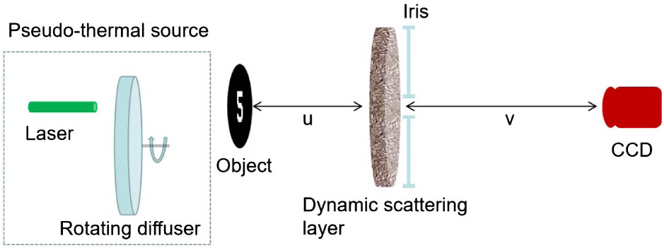
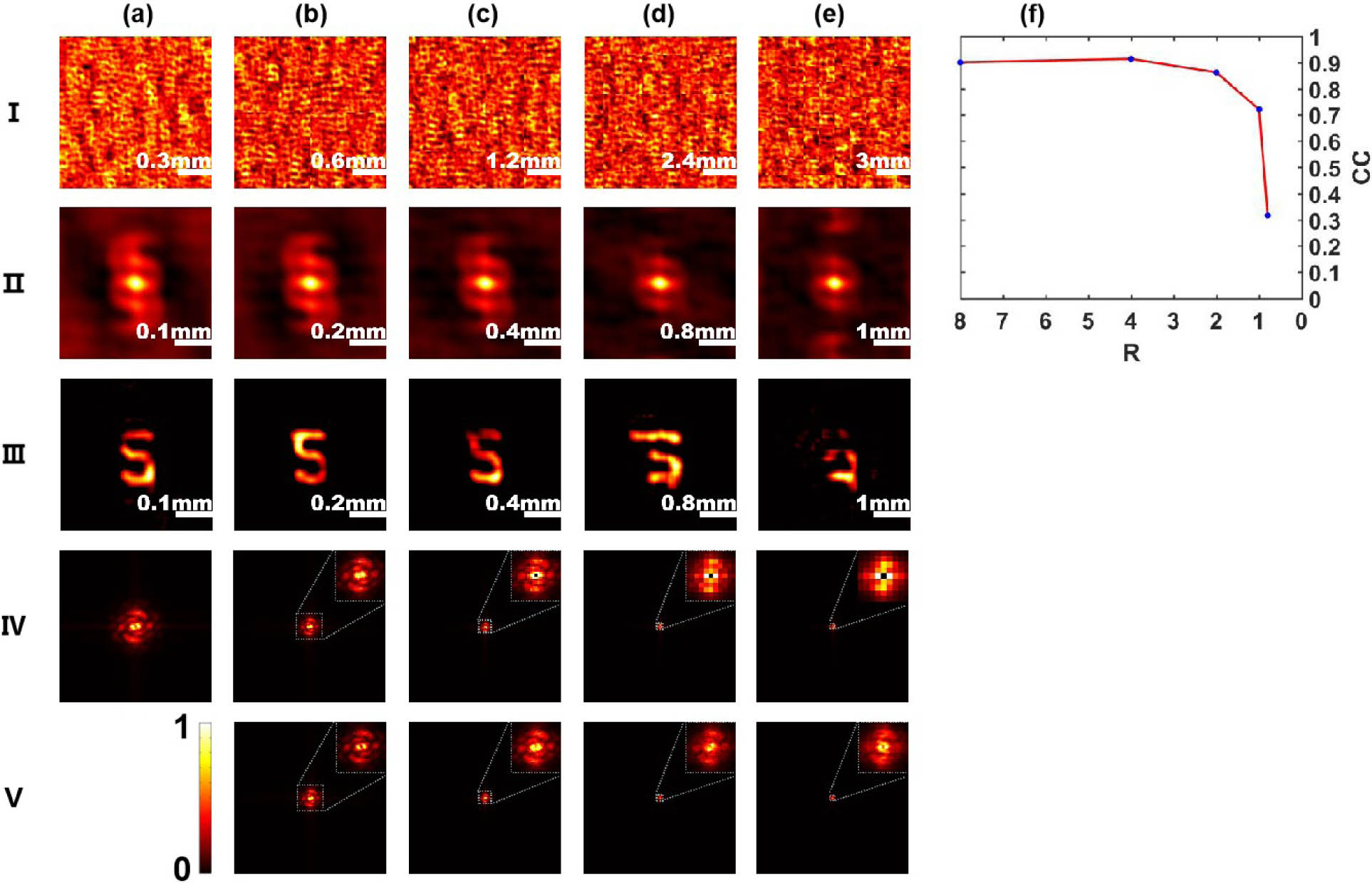
Fig. 3. Experimental setup. u and v are distances from the object and the camera to the scattering layer, respectively.

下载图片 查看所有图片

Fig. 4. Experimental results. Rows I, II, and III correspond to R=10.8, 5.4, and 3.6, respectively. (a) Examples of captured speckle patterns, and (b) the corresponding autocorrelations of (a). (c) The power spectra of (a), (d) the averaged power spectra, and (e) the images reconstructed from (d). (f) The stitched speckle patterns at different sampling ratios and numbers of frames: R=10.8, 4×4 frames (row I); R=5.4, 8×8 frames (row II); and R=3.6, 12×12 frames (row III), respectively. (g) The corresponding power spectra of (f), and (h) the images reconstructed from (g). (II,i) The autocorrelation and (III,i) the frequency spectrum of (I,i), the object. The inserts in rows II and III, and columns (c), (d), and (h) show zoom-ins of the center dash squares.

下载图片 查看所有图片

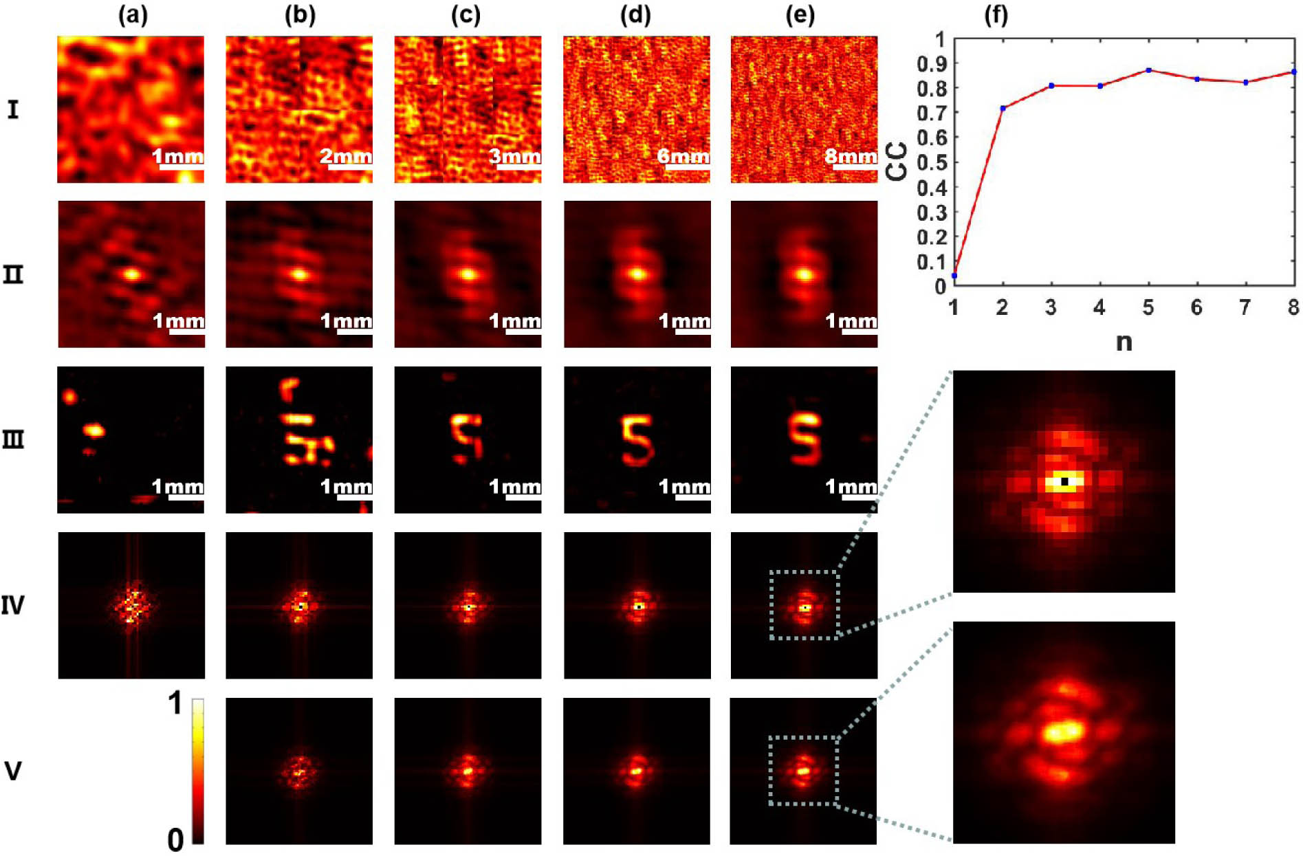
Figure 5 shows the simulations of the influence of the stitching number on the autocorrelation and reconstruction quality. In the simulation, u=6cm, v=30cm, rO=160μm, rD=1.6mm, and thus R=2. The correlation coefficient (CC) between the recovered image and the amplified target of the same size is used to quantify the reconstruction quality. CC=∑i∑j(Aij−A¯)(Bij−B¯)[∑i∑j(Aij−A¯)2][∑i∑j(Bij−B¯)2], where Aij, Bij are the individual pixel intensities of the reconstructed image and the amplified target, respectively, and A¯, B¯ are the mean intensities, respectively. Obviously, the stitching method can suppress the noise and increase the resolution in the power spectrum for more details (the autocorrelation image of the stitching method has more pixels than that of the autocorrelation summing method, which thus leads to a finer Fourier spectrum, as shown in Figs. 5(IV) and 5(V), and local magnification diagrams). As the stitching number n increases, the quality of the speckle autocorrelation and reconstructed image improves. However, the improvement speed gradually decreases, so there is no need to pursue R to be as large as possible since the gain is trivial when the equivalent R∪ is big enough.

Fig. 5. Simulation results of different stitching numbers at R=2. Row I. (a) A single original speckle pattern; and (b) 4, (c) 9, (d) 36, and (e) 64 original patterns stitched together equally in two directions. Row II. The autocorrelations corresponding to I. Row III. The respective images reconstructed. Row IV. The averaged power spectra of 1, 4, 9, 36, and 64 frames of the original patterns. Row V. The corresponding power spectra of row I. (f) The evolution of the correlation coefficient with stitching number n. In rows IV and V, all have the same spectrum range because of the same pixel pitch. However, the power spectra of the stitched patterns have a higher resolution determined by the array size, which can be seen clearly from the amplified dash squares.

下载图片 查看所有图片

Next, we investigated the relationship between the image quality and R under the same equivalent sampling ratio R∪. The simulations were done at fixed rO=160μm, rD=0.64mm, and u=6cm, but different v=3,6,12,24,30cm, corresponding to R=8,4,2,1,0.8, respectively. We chose the speckle pattern of R=8 as a reference and stitched each set of speckle patterns of R=4,2,1,0.8 into synthesized patterns that have the same R∪ as the reference one, i.e., stitching 2×2, 4×4, 8×8, and 10×10 small original speckle patterns into a big one. Figure 6 shows the simulation results. When R≥1, the autocorrelation quality can be improved by stitching, and the image can be reconstructed completely. However, for R=0.8, we cannot obtain a complete structure of the autocorrelation or power spectrum to recover the image. As is known with lack of axial resolution, speckle autocorrelation imaging is similar to pinhole imaging. If we see the scattering layer as countless pinholes with randomly shifted centers, the detected speckle pattern is a superposition of all the shifted images of the object. When the entire image is located within the sensor area, its autocorrelation and power spectrum are the same even though its center is shifted and can be added coherently. Otherwise, the autocorrelation and power spectrum will be changed, and summing this part may be not helpful in image reconstruction. Thus, in order to make sure at least one complete image is obtained, the sampling ratio R should not be less than 1, i.e., the valid detection area radius cannot be smaller than vurO. In other words, the angle of the detector should not be smaller than the angle of the target when viewing the scattering layer.

Fig. 6. Simulation results of different sampling ratios R. Row I. (a) A speckle pattern at R=8, and stitched speckle patterns of different sampling ratios and numbers of frames: (b) R=4, 2×2 frames; (c) R=2, 4×4 frames; (d) R=1, 8×8 frames; and (e) R=0.8, 10×10 frames, respectively. Row II. Autocorrelations corresponding to I. Row III. Reconstructed images, respectively. Row IV. Averaged power spectra. Row V. Corresponding power spectra of I (b)–(e). (f) The evolution of the correlation coefficient versus sampling ratio R. Again, all power spectra in rows IV and V have the same spectral range but different resolutions.

下载图片 查看所有图片

In Fig. 6(f), the CC curve has a steep falling around R=1. A possible explanation is that at the edges of each detected speckle pattern some speckle grains are broken; for a smaller R, the fraction of broken speckle grains is large, which results in less independent speckle grains in the ensemble average, and hence a deteriorated image quality.

In this Letter, we should keep in mind that in the experiment the exposure time of the CCD camera should be less than the decorrelation time, and the speckle recording must comply with the Nyquist sampling law. In the above experiments and simulations, each reconstruction is carried out under the same number of iterations of the phase retrieval algorithm. Due to the randomness caused by phase retrieval algorithm, the image quality could fluctuate slightly. Because of the background noise, the actual stitching number required in the experiment is always larger than that in the simulation to achieve a comparable reconstruction quality under the same sampling ratio. Compared to simple averaging, stitching can suppress the background noise, and simultaneously enhance the resolution in the frequency domain to see more details, which is critical to reconstruct the image, especially for a small sampling ratio R.

Different from solid bodies like rotating ground glass disks, white paint, tissue mimicking phantoms, and biological tissues, the decorrelation time of fog and polluted water is orders-of-magnitude smaller, with a characteristic time of microseconds^[36]. By utilizing the shorter decorrelation time, an automatic stitching speckle pattern can be realized by scanning over an array of cheap industrial CCD cameras, which is competitive in cost, dynamic range, and extensibility compared to a billion-pixel camera. It provides an alternative real-time imaging solution. In addition, the stitching method can also apply to a moving object, as long as the object is approximately stationary within each exposure time and the object itself is within the memory effect range.

In conclusion, we reveal a relationship between detector and object sizes for the minimum requirement to ensure image reconstruction by defining a sampling ratio R, and propose a method to stitch speckle patterns recorded under a large image distance v to obtain a speckle pattern with an equivalent large sampling ratio R∪ by exploiting the dynamic feature of the scattering medium. In addition to suppressing the background noise, it can simultaneously enhance the frequency-spectrum resolution for a better image reconstruction. In this way we can reconstruct the image of the object under a larger v with a cheap detector. The lower threshold R=1 to reconstruct a complete image is given based on the simulation, which, in practice, would be a little larger than 1 due to the existence of noise. Our method can reduce the dependence on hardware and expands the application scope of speckle autocorrelation imaging. It has great prospects in many practical applications such as navigation, remote sensing, and undersea detection.

References

[1] GoodmanJ. W., Introduction to Fourier Optics (Roberts and Company Publishers, 2005).
[2] GoodmanJ. W., Speckle Phenomena in Optics: Theory and Applications (Roberts and Company Publishers, 2007).
[3] AlfanoR.LiangX.WangL.HoP., Science264, 1913 (1994).SCIEAS0036-8075
[4] HelmchenF.DenkW., Nat. Methods2, 932 (2005).1548-7091
[5] Andersson-EngelsS.BergR.SvanbergS.JarlmanO., Opt. Lett.15, 1179 (1990).OPLEDP0146-9592
[6] LaiP.WangL.TayJ. W.WangL. V., Nat. Photon.9, 126 (2015).NPAHBY1749-4885
[7] HorstmeyerR.RuanH.YangC., Nat. Photon.9, 563 (2015).NPAHBY1749-4885
[8] VellekoopI. M.LagendijkA.MoskA., Nat. Photon.4, 320 (2010).NPAHBY1749-4885
[9] VellekoopI. M., Opt. Express23, 12189 (2015).OPEXFF1094-4087
[10] CaoX.GuanM.XiaL.SangX.ChenZ., Chin. Opt. Lett.15, 120901 (2017).CJOEE31671-7694
[11] AziziL.ZarychtaK.EttoriD.TinetE.TualleJ.-M., Opt. Express17, 12132 (2009).OPEXFF1094-4087
[12] AndreoliD.VolpeG.PopoffS.KatzO.GrésillonS.GiganS., Sci. Rep.5, 10347 (2015).SRCEC32045-2322
[13] KimM.ChoiW.ChoiY.YoonC.ChoiW., Opt. Express23, 12648 (2015).OPEXFF1094-4087
[14] PopoffS.LeroseyG.CarminatiR.FinkM.BoccaraA.GiganS., Phys. Rev. Lett.104, 100601 (2010).PRLTAO0031-9007
[15] ChaigneT.KatzO.BoccaraA. C.FinkM.BossyE.GiganS., Nat. Photon.8, 58 (2014).NPAHBY1749-4885
[16] ZhuangB.XuC.GengY.ZhaoG.ChenH.HeZ.WuZ.RenL., Chin. Opt. Lett.16, 041102 (2018).CJOEE31671-7694
[17] YaqoobZ.PsaltisD.FeldM. S.YangC., Nat. Photon.2, 110 (2008).NPAHBY1749-4885
[18] SiK.FiolkaR.CuiM., Nat. Photon.6, 657 (2012).NPAHBY1749-4885
[19] HsiehC.-L.PuY.GrangeR.LaporteG.PsaltisD., Opt. Express18, 20723 (2010).OPEXFF1094-4087
[20] MaC.XuX.LiuY.WangL. V., Nat. Photon.8, 931 (2014).NPAHBY1749-4885
[21] XuX.LiuH.WangL. V., Nat. Photon.5, 154 (2011).NPAHBY1749-4885
[22] WangY. M.JudkewitzB.DiMarzioC. A.YangC., Nat. Commun.3, 928 (2012).NCAOBW2041-1723
[23] ZhangP.LiuD.YangA.ZhuJ., Chin. Opt. Lett.17, 070901 (2019).CJOEE31671-7694
[24] EdreiE.ScarcelliG., Sci. Rep.6, 33558 (2016).SRCEC32045-2322
[25] BertolottiJ.Van PuttenE. G.BlumC.LagendijkA.VosW. L.MoskA. P., Nature491, 232 (2012).
[26] CuaM.ZhouE. H.YangC., Opt. Express25, 3935 (2017).OPEXFF1094-4087
[27] KatzO.HeidmannP.FinkM.GiganS., Nat. Photon.8, 784 (2014).NPAHBY1749-4885
[28] NewmanJ. A.LuoQ.WebbK. J., Phys. Rev. Lett.116, 073902 (2016).PRLTAO0031-9007
[29] LiuH.WangX.GaoJ.YuT.HanS., J. Innov. Opt. Heal. Sci.12, 1942001 (2019).
[30] FreundI.RosenbluhM.FengS., Phys. Rev. Lett.61, 2328 (1988).PRLTAO0031-9007
[31] JudkewitzB.HorstmeyerR.VellekoopI. M.PapadopoulosI. N.YangC., Nat. Phys.11, 684 (2015).NPAHAX1745-2473
[32] OsnabruggeG.HorstmeyerR.PapadopoulosI. N.JudkewitzB.VellekoopI. M., Optica4, 886 (2017).
[33] YangW.LiG.SituG., Sci. Rep.8, 9614 (2018).SRCEC32045-2322
[34] FienupJ. R., Opt. Lett.3, 27 (1978).OPLEDP0146-9592
[35] FienupJ. R., Appl. Opt.21, 2758 (1982).APOPAI0003-6935
[36] MaretG.WolfP., Zeitschrift für Physik B Condensed Matter65, 409 (1987).
Xin Wang, Honglin Liu, Meijun Chen, Zhentao Liu, Shensheng Han. Imaging through dynamic scattering media with stitched speckle patterns[J]. Chinese Optics Letters, 2020, 18(4): 042604.
本文已被 1 篇论文引用
被引统计数据来源于中国光学期刊网
引用该论文: TXT   |   EndNote
相关论文
加载中...
关于本站 Cookie 的使用提示
中国光学期刊网使用基于 cookie 的技术来更好地为您提供各项服务,点击此处了解我们的隐私策略。 如您需继续使用本网站,请您授权我们使用本地 cookie 来保存部分信息。
全站搜索
您最值得信赖的光电行业旗舰网络服务平台!